Unlike differentiation, there is no systematic method for integrating any function given in closed form, but rather a library of calculation techniques (i.e. a calculus) that can be applied ad hoc to specific functions. (Although see also the Risch algorithm for a close miss.)
As a simple example, consider
![]()
which can be solved through various classical techniques, or verified
by computing the derivative of ![]() . In fact we’ll find a use for this
integral in an upcoming entry. However the integral
. In fact we’ll find a use for this
integral in an upcoming entry. However the integral
![]()
is less obvious, as the corresponding indefinite integral is not easily solvable.
I saw this latter integral presented as an example that is amenable to the use of contour integration methods. However, my lack of familiarity with such method leads me to favor the use of partial fractions for this problem. But when I worked through the problem with partial fractions, it became clear that here the two techniques are really the same in disguise.
Let’s walk through the steps of computing
![]()
using both partial fractions and contour integration. Here we take
![]() to be a monic polynomial of degree at least 2,
with no repeated roots and no real roots, although in general the
following steps equally apply to any quotient of polynomials. Let
to be a monic polynomial of degree at least 2,
with no repeated roots and no real roots, although in general the
following steps equally apply to any quotient of polynomials. Let
![]()
We need to find ![]() such that
such that
![]()
this is called the partial fraction decomposition of ![]() . Multiplying both sides by
. Multiplying both sides by ![]() gives an equality of polynomials in
gives an equality of polynomials in ![]() that needs to hold for all
that needs to hold for all ![]() ; we can regard this as a system of
; we can regard this as a system of ![]() linear equations with
linear equations with ![]() unknowns. However, the easier way to solve this is
to evaluate both sides at
unknowns. However, the easier way to solve this is
to evaluate both sides at ![]() , as that makes all but one term on the
right go to zero. We get
, as that makes all but one term on the
right go to zero. We get
![]()
(which you can verify by expanding ![]() ). These
). These ![]() are the residues of
are the residues of ![]() at each of its poles.
at each of its poles.
Now
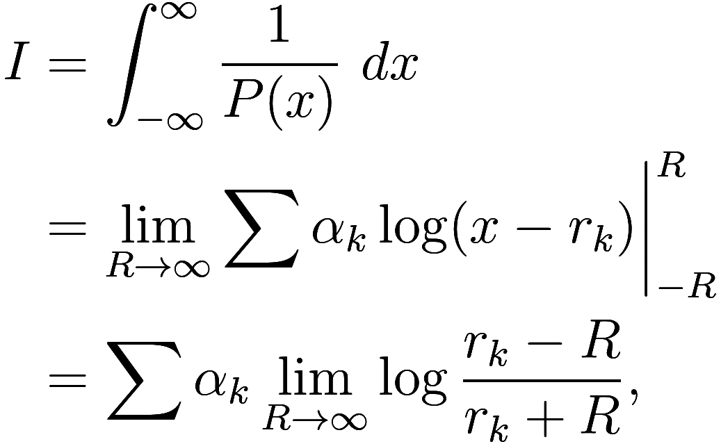
so it remains to calculate the limit of this log expression. As we
are taking log of complex numbers, we need to be careful to choose a
branch cut of log that is not crossed by the line from ![]() to
to ![]() . The standard choice for the branch cut,
the negative real axis, works for this purpose as we have specified that
none of the
. The standard choice for the branch cut,
the negative real axis, works for this purpose as we have specified that
none of the ![]() are real. (If any of the
are real. (If any of the ![]() are real we would need to deal with integrating
through a singularity in
are real we would need to deal with integrating
through a singularity in ![]() .)
.)
We know that
![]()
so we need to know the magnitude ![]() of
of ![]() for large
for large ![]() , and its angle
, and its angle ![]() . In the limit of large
. In the limit of large ![]() , its magnitude goes to 1. The angle depends on
whether the imaginary part of
, its magnitude goes to 1. The angle depends on
whether the imaginary part of ![]() is positive. If
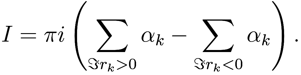
is positive. If ![]() , then the angle of
, then the angle of ![]() approaches
approaches ![]() ; otherwise
; otherwise ![]() . Thus we have
. Thus we have
This can be simplified slightly: let us show that the sum of the
residues ![]() is zero. In the next section we will see
an immediate way to prove this. For now, note that in our equation
is zero. In the next section we will see
an immediate way to prove this. For now, note that in our equation
![]()
that ![]() is the coefficient of the
is the coefficient of the ![]() term on the left, and
term on the left, and ![]() is the coefficient of the
is the coefficient of the ![]() term on the right. Then it follows
that
term on the right. Then it follows
that
![]()
We can calculate ![]() using the residue
theorem, which states that
using the residue
theorem, which states that
![]()
where ![]() is a meromorphic function and the sum on the
right is of the residues of
is a meromorphic function and the sum on the
right is of the residues of ![]() at each of the poles inside of the contour. The
definition
of residue is the unique value such that the difference
at each of the poles inside of the contour. The
definition
of residue is the unique value such that the difference
![]()
has an antiderivative in a small punctured disc around ![]() . (It is fine if
. (It is fine if ![]() has a pole of order higher than 2, as integrating
has a pole of order higher than 2, as integrating
![]() only creates a branch cut when
only creates a branch cut when ![]() exactly. Thus the residue is the coefficient
of the
exactly. Thus the residue is the coefficient
of the ![]() term.)
term.)
The residue theorem is a direct consequence of Cauchy’s
theorem, which states that the contour integral of a holomorphic
function is zero. Suppose we want to use this to compute a contour
integral that goes around some poles. Then by Cauchy’s theorem we can
write ![]() as a sum of contour integrals, one for each
pole, each of them going in a circle of arbitrarily small radius around
that pole. Then, by definition of residue, we can replace these
integrals with ones of the form
as a sum of contour integrals, one for each
pole, each of them going in a circle of arbitrarily small radius around
that pole. Then, by definition of residue, we can replace these
integrals with ones of the form ![]() that can be computed easily to
give the desired result.
that can be computed easily to
give the desired result.
So what are these residues for the function ![]() ? Unsurprisingly, the residue of
? Unsurprisingly, the residue of ![]() at
at ![]() is
is ![]() , as can be seen from the equation
, as can be seen from the equation
![]()
together with the definition of residue. Then if we choose a contour to integrate around, the residue theorem tells us that
![]()
where the sum is taken over ![]() such that
such that ![]() is inside of the contour.
is inside of the contour.
It remains to choose a suitable contour. First, imagine taking a
large circle of radius ![]() around the origin, with
around the origin, with ![]() , and let
, and let ![]() be the value of the
integral.
be the value of the
integral.
In the limit ![]() , the length of the path being
integrated along grows like
, the length of the path being
integrated along grows like ![]() , but the integrand
, but the integrand ![]() shrinks like
shrinks like ![]() , so
, so ![]() . But by the residue theorem,
. But by the residue theorem, ![]() only depends on which poles are inside the
contour, which is independent of
only depends on which poles are inside the
contour, which is independent of ![]() , so
, so ![]() . Therefore
. Therefore
![]()
where the sum on the right is over all ![]() . This gives us again our result that the
residues have a sum of zero, which we needed in the previous
section.
. This gives us again our result that the
residues have a sum of zero, which we needed in the previous
section.
Now we return to computing ![]() and choose a semicircular contour, running along
the real axis from
and choose a semicircular contour, running along
the real axis from ![]() to
to ![]() , and then following a semicircular arc in the
upper-half plane; let
, and then following a semicircular arc in the
upper-half plane; let ![]() be the value of this integral.
be the value of this integral.
![]() is a sum of two components, for the two parts
of the path being integrated along. As with
is a sum of two components, for the two parts
of the path being integrated along. As with ![]() , the semicircular arc component goes to 0 in
the limit of large
, the semicircular arc component goes to 0 in
the limit of large ![]() . And again as before, the value of
. And again as before, the value of ![]() is independent of
is independent of ![]() for large
for large ![]() , so
, so
![]()
Then we compute ![]() with the residue theorem, giving
with the residue theorem, giving
![]()
where the sum is over roots ![]() in the upper-half plane, in agreement with the
result of the computation with partial fractions.
in the upper-half plane, in agreement with the
result of the computation with partial fractions.
Step-by-step, the two methods involve nearly the same operations.
With contour integration, we took advantage of Cauchy’s theorem and that
![]() is holomorphic to choose contours that are
convenient instead of being committed to integrating along the real
axis. This made it trivial to find the sum of the residues, and also
simplified the task of integrating the functions
is holomorphic to choose contours that are
convenient instead of being committed to integrating along the real
axis. This made it trivial to find the sum of the residues, and also
simplified the task of integrating the functions ![]() . When integrating along the real
axis, we had to do some geometric reasoning about whether the imaginary
part of
. When integrating along the real
axis, we had to do some geometric reasoning about whether the imaginary
part of ![]() is positive or negative, but using Cauchy’s
theorem we can instead integrate in a circle around
is positive or negative, but using Cauchy’s
theorem we can instead integrate in a circle around ![]() , which was elided as “easy” in our sketch of
the proof of the residue theorem.
, which was elided as “easy” in our sketch of
the proof of the residue theorem.
Otherwise, the two methods are identical. I was surprised that to calculate the residues by directly applying the definition of “residue” as given on Wikipedia requires first finding the partial fraction decomposition. Of course, while there are various theorems that hasten the calculation of the residues in practice, these are equally applicable to hastening the partial fraction decomposition.
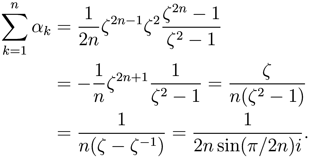
Let us work through the specific example ![]() . If
. If ![]() is the primitive
is the primitive ![]() th root of unity
th root of unity ![]() , then the roots of
, then the roots of ![]() are
are
![]()
for ![]() , of which the first
, of which the first ![]() have positive imaginary part. As
have positive imaginary part. As ![]() , we get
, we get
![]()
so
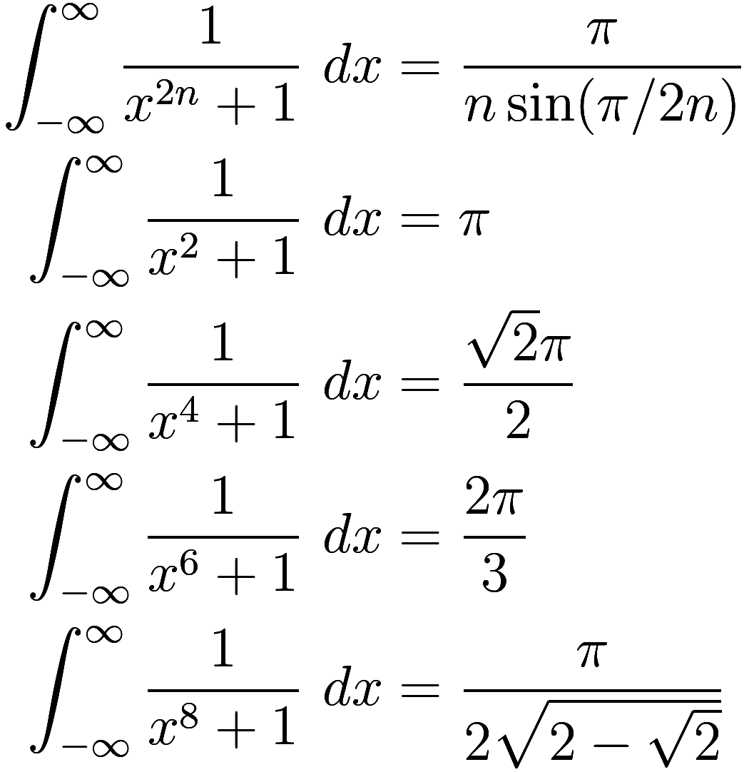
Finally we get
Follow RSS/Atom feed for updates.