Temperature part 1: What is negative temperature?

2022 April 05

Part 1: What is negative temperature?
Part 2: What is temperature? (coming)
Part 3: Why does entropy increase? Resolving Loschmidt’s paradox. (coming)
Part 4: Temperature of black holes (coming?)

This is a four-part exploration of topics related to temperature. In part 1 I start by asking about the units in which we measure temperature and end up investigating a model that permits negative temperature. We are left with some foundational questions unresolved, and in part 2 we must retreat to the very basics of statistical mechanics to justify the concept of temperature. Part 3 edges into philosophical grounds, attempting to justify the central assumption of statistical mechanics that entropy increases with time, with implications on the nature of time itself. Finally in part 4 I jump topics to black holes to look at their unusual thermodynamic properties.

Units for describing temperature

Our bodies are able to directly sense variations in the temperature of objects we touch, which forms the motivation of our understanding of temperature. The first highly successful quantified measurements of this property came with the invention of the mercury thermometer by Fahrenheit, along with his scale temperatures were measured on. He chose to use higher numbers to represent the sensation we call “hotter”.

With the discovery of the ideal gas laws came the realization that temperature is not “affine”, by which I mean that the laws of physics are not the same if you translate all temperatures up or down a fixed amount. In particular, there exists a minimum temperature. The Fahrenheit and Celsius scales were designed in ignorance of this fact, but they were already well-established by that point and continued to be used for historical reasons. Kelvin decided to address this problem by inventing a new scale, in which he chose to use zero for the minimum temperature.

Now with our modern theory of statistical mechanics, temperature is no longer just a thing that thermometers measure but is defined in terms of other thermodynamic properties:

$T = \frac {dU}{dS}$

where $T$ is the temperature of a system (in Kelvin), $U$ is its energy, and $S$ is its entropy. We will skip past the question of “what is energy” (not because it is easy, but because there is no good answer) to quickly define entropy. While in classical thermodynamics entropy was originally defined in terms of temperature (via the above equation), in statistical mechanics entropy is defined as a constant times the amount of information needed to specify the system’s microstate:

$S = -k_B \log \Omega$

where $\Omega$ is the number of possible microstates (assuming uniform distribution), and we will return to $k_B$ in just a moment.

Unfortunately there remain two more inelegancies with this modern definition of temperature. The first is that the proportionality constant is a historial accident of Celsius’s choice to use properties of water to define temperature. Indeed, temperature is in the “wrong” units altogether. We like to think of temperature as related to energy somehow. It turns out, the Boltzmann constant accomplishes exactly that:

$k_B = 1.380649 \cdot 10^{-23} \text{ J / K}$

The $k_B$ that appeared in the definition of entropy was just there to get the units to agree with historical usage – if we dropped it, we could be measuring temperature in Joules instead! Well, more likely in zeptoJoules, since room temperature would be a bit above $4 \cdot 10^{-21}$ J. In summer we’d talk about it being a balmy 4.2 zeptoJoules out, but 4.3 would be a real scorcher.

(When measuring temperature in Joules it should not be confused with thermal energy, which is also in Joules! The former is an intensive quantity, while the latter is an extensive quantity. Maybe it is for the best that we have a special unit for temperature, just to avoid this confusion.)

Thermodynamic beta

To introduce what I perceive to be the second inelegancy of the modern definition of temperature, I will walk through a worked example of calculating the temperature of a simple system.

Suppose we have $N$ magnetic particles in an external magnetic field. Each particle can either be aligned with the field, which I will call “spin down”, or against it, i.e. “spin up”; a spin up particle contains $E$ more energy than one that is spin down. This is the Ising model with no energy contained in particle interactions.

A microstate is a particular configuration of spins. The ground state or lowest-energy state of the model is the configuration that has all spins down. If some fraction $p$ of the spins are up, then the energy is

$U = pNE.$

We need to calculate the distribution of possible microstates that correspond to a given energy level. Certainly we can find the number $\Omega$ of microstates with $pN$ up spins, but are they are equally likely to occur? Though it may seem strange, perhaps depending on the geometry of the system certain particles may have correlated spins causing certain microstates to be more probable than others.

In fact, with certain minimal assumptions, the distribution over all possible microstates is necessarily uniform. We suppose that nearby particles in the system can interact by randomly exchanging their spins. Furthermore distant particles can exchange spins via some chain of intermediate particles: if not, the system would not have a single well-defined temperature, but each component of the system would have its own temperature.

Thus the system varies over all configurations with $pN$ up spins: it remains to see that the distribution is uniform. The particle interaction is adiabatic and time reversible, so the probability that two particles exchange spin is independent of what their spins are, and therefore it can be shown that the Markov chain for the state transition converges to a uniform distribution over all accessible configurations. That is, the distribution of microstates is uniform on a sufficiently long time period; on a shorter timescale the system does not have a well-defined temperature.

The number of configurations with $N$ particles and $pN$ up spins is $\Omega = \binom {N}{pN}$ , and $\log \Omega$ is the information needed to specify which microstate we are in. Thus the entropy is

$\begin{aligned} S &= k_B \log \binom {N}{pN} \\ &= k_B \log \frac {N!}{(pN)!((1 - p)N)!} \\ &\approx k_B N (\log N - p \log pN - (1 - p) \log ((1 - p)N)) \\ &= -k_B N (p \log p + (...$

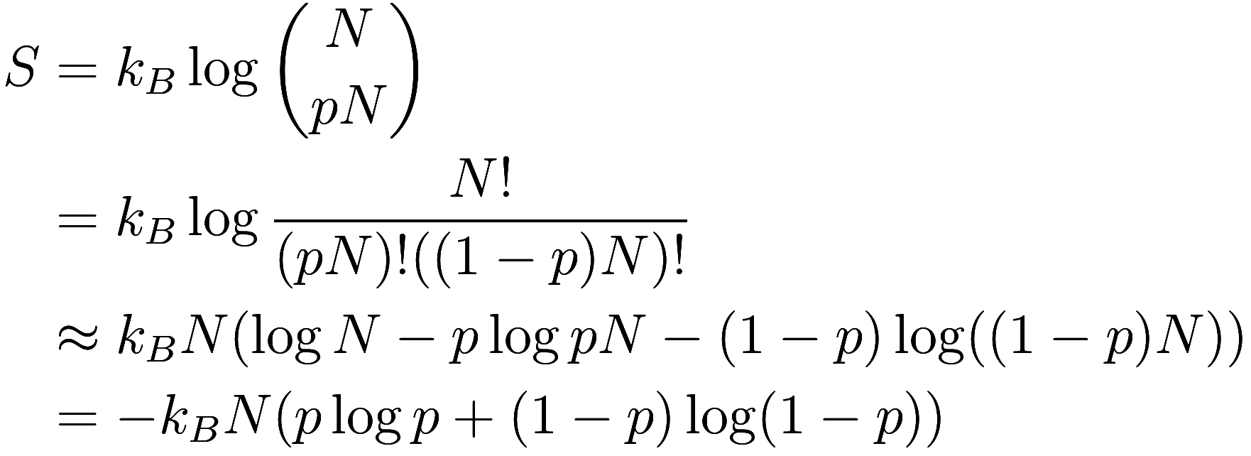
where we have used Stirling’s approximation. (Note that when using Stirling’s approximation on binomial coefficients, the second term in the approximation always cancels out.)

What is the point of all this faffing about with microstates and our information about them? After all, with temperature defined in this way, temperature is not a strictly physical property but rather depends on our information about the world. However at some point we would like to get back to physical phenomena, like the sensation of hot or cold that we can feel directly: this connection will be justified in part 2.

Now

$\frac {dS}{dp} = k_B N (\log (1 - p) - \log p)$

and $p = U / (NE)$ , so $dp / dU = 1 / (NE)$ and

$\begin{aligned} \frac {dS}{dU} &= \frac {k_B}{E} (\log (1 - p) - \log p) \\ T = \frac {dU}{dS} &= \frac {E}{k_B} \cdot \frac 1{\log (1 - p) - \log p}. \end{aligned}$

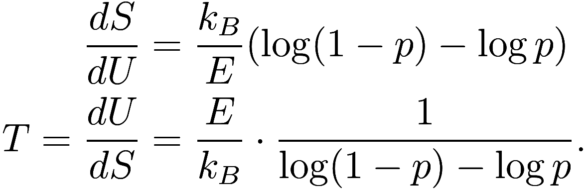
Alright, so what have we learned? Let’s plug in some values for $p$ and see. First, for the ground state $p = 0$ , we have $\log p = \infty$ so therefore we get $T = 0$ (in Kelvin). That’s not a big surprise, that the lowest energy state is also absolute zero.

What about the highest energy state $p = 1$ ? Now we have $\log (1 - p) = \infty$ so again $T = 0$ . Wait, what?

Maybe this model just thinks everything is absolute zero? How about the midpoint $p = 1/2$ : then $\log p - \log (1 - p) = 0$ so $T = \infty$ . Great.

We can just graph this so we can see what is really going on:

(Note the temperature is only defined up to a scalar constant that depends on the choice of $E$ .) As the system gets hotter, the temperature starts from +0 Kelvin, increases through the positive temperatures, hits $\infty$ K, increases through the negative temperatures, and then reaches -0 Kelvin, which is the hottest possible temperature.

So zero Kelvin is two different temperatures, both the hottest and coldest possible temperatures. Positive and negative infinity are the same temperature. (Some sources in the literature I read incorrectly state that positive and negative infinity are different temperatures.) Negative temperatures are hotter than positive temperatures.

This is quite a mess, but one simple change in definition fixes everything, which is to use inverse temperature, also called thermodynamic beta or coldness:

$\beta = \frac 1{k_B T} = \frac 1{k_B} \frac {dS}{dU}.$

$\beta$ has units of inverse Joules, but thinking of temperature from an information theory perspective and using 1 bit = $\log 2$ , we can equate room temperature to about 45 gigabytes per nanoJoule. This is a measure of how much information is lost (i.e. converted into entropy) by adding that much energy to the system.

With $\beta$ , the coldest temperature is $+\infty$ and the hottest temperature is $-\infty$ . Ordinary objects (including all unconfined systems) have positive temperatures while exotic systems like the magnetic spin system we considered above can have negative temperatures. If you prefer hotter objects to have a higher number on the scale, you can use $-\beta$ , but then ordinary objects have negative temperature.

Negative temperature

The magnetic spin system of the previous section is a classic introduction to statistical mechanics, but as we’ve seen it admits the surprising condition of negative temperature. What does it mean for an object to have negative temperature, and can this happen in reality?

The first demonstration of a negative temperature was in 1951 by Purcell and Pound, with a system very similar to the magnetic spin system we described. They exposed a LiF crystal to a strong 6376 Gauss magnetic field, causing the magnetized crystal to align with the imposed field. The magnetic component of the crystal had a temperature near room temperature at this point. Then, reversing the external field, the crystal maintained its original alignment, causing its temperature to be near negative room temperature, then cooling to room temperature through $\infty$ K over the course of several minutes. As it cooled, it dissipated heat to its surroundings.

Why did it cool off? On a time scale longer than it takes for the LiF’s magnet to reach internal thermal equilibrium, but shorter than it takes to cool off, the LiF’s magnet and the other forms of energy (e.g. molecular vibrations) within the LiF crystal are two separate thermal systems, each with their own temperature. However these two forms of energy can be exchanged, and on a time scale longer than it takes for them to reach thermal equilibrium with each other they can be treated as a single system with some intermediate temperature. As the molecular vibrations had a positive temperature, and the magnetic component had a negative temperature, thermal energy flowed from the latter to the former.

Consider more generally any tangible object made of ordinary atoms and molecules in space. The object will contain multiple energy states corresponding to various excitations of these atoms, such as vibrations and rotations of molecules, electronic excitations, and other quantum phenomena. For these excitations, the entropy increases rapidly with energy, so the corresponding temperatures will always be positive. Whatever other forms of energy the object exhibits, they will eventually reach equilibrium with the various atomic excitations, and thus converge on a positive temperature.

While such an object will exhibit increasing entropy with energy on the large scale, maybe it is possible for it to have a small-scale perturbation in entropy and thus a narrow window with negative temperatures. Perhaps, but some of the atomic excitations are very low energy, and thus they have a gradually increasing entropy that is smooth even to quite a small scale. Only under some very unusual circumstance could that object have negative temperatures.

None-the-less in 2012 researchers were able to bring a small cloud of atoms to a negative temperature in their motional modes of energy. I read the paper but didn’t really understand it.

As an aside – what if some exotic object had a highest energy state but no lowest energy state? This object could only have negative temperatures, would always be hotter than any ordinary objects it was in contact with, so would perpetually have thermal energy flowing from it.

(An object with no highest or lowest energy state could never reach internal thermal equilibrium, wouldn’t have a well-defined temperature, and its interactions with other objects couldn’t be represented as an average of small-scale phenomena, making statistical mechanics inapplicable.)

Lasers

However, negative temperatures are closely related to a phenomenon which is essential in the functioning of an important modern technology: lasers! Lasers produce light when excited electrons in the lasing medium drop to a lower energy level, emitting a photon. While an excited electron can spontaneously emit a photon, lasers produce light through stimulated emission of an excited electron with a photon of the matching wavelength: the stimulated photon is synchronized exactly with the stimulating photon, which is why lasers can produce narrow, coherent beams of light. However, the probability that a photon stimulates emission from an excited electron is equal to the probability that the photon would be absorbed by an unexcited electron, so for a beam of light to occur the majority of the electrons must be excited.

This is an example of population inversion, where a higher-energy state has greater occupancy than a lower-energy state. Population inversion is a characteristic phenomenon of negative temperatures: an object at thermal equilibrium with a positive temperature will always have occupancy decrease with energy, while at negative temperature it will always have occupancy increase with energy. (At infinite temperature, occupancy of all states is equal.)

But is the lasing medium at thermal equilibrium? Certainly we have to consider a short enough time scale for the electronic excitations to be treated separately from the motional energy modes. However even considering only electronic modes, modern lasers do not operate at thermal equilibrium. Originally lasers used three energy levels (a ground state and two excited states), for which it would have been debatable whether calling the lasing medium “negative temperature” is appropriate. Now, most lasers use four (or more) energy levels due to their far greater efficiency.

Such a laser has two low-energy levels, and two high-energy levels. The narrow transitions (between the bottom two or the top two levels) are strongly coupled with vibrational or other modes, so electrons rapidly decay to the lower of the two. As a result, there is a very low occupancy in the second-lowest energy level, making it easy to generate a strong population inversion between the two middle energy levels, which is the lasing transition. Thus the laser still operates at positive (but non-equilibrium) temperature, as most electrons remain in the ground state even when a population inversion between two higher levels is created.

Appendix: Proof of uniformity of distribution in microcanonical ensemble

We claimed that, under reasonable physical assumptions, the spin system with $pN$ up spins will eventually be equally likely to be in any of the $\binom {N}{pN}$ such configurations. (A particular configuration of up / down spins is called a microstate, and the collection of all microstates with the same energy is called a microcanonical ensemble (MCE).) This is intuitively sensible since any particular spin goes on a random walk over all particles, and thus any particular particle is eventually equally likely to have any of the starting spins. However I found rigorously proving this more involved than I thought, and I haven’t seen any similar argumentation elsewhere, so let’s work out all the details.

Any two “nearby” particles can exchange spins with some probability, not necessarily equal for all such pairs. Let us discretize so that in each time step either 0 or 1 such exchanges happen. The graph of particles with edges for nearby particles is connected: otherwise the system would actually be multiple unrelated systems. There are finitely many microstates in the MCE, and we can get from any one to any other in at most $N^2$ time steps with positive probability, for example using bubble sort.

Let $Q$ be the state transition matrix. In the language of Markov chains, we have a time-homogeneous Markov chain (because the probability of a swap does not depend on the spins involved) which is irreducible (i.e. any state can get to any other) and is aperiodic (a consequence of the identity transition having positive probability) and thus ergodic (irreducible and aperiodic). First we would like to establish that the Markov chain converges to a stationary distribution: this is effectively exploring the behavior of $Q^k$ for large $k$ .

The behavior of $Q^k$ is dominated by its largest eigenvalue. Since all elements of $Q^{N^2}$ are positive real numbers, by the Perron-Frobenius_theorem it has a positive real eigenvalue which has strictly larger magnitude than any other eigenvalue, and which has an eigenspace of dimension 1, and furthermore an eigenvector $v$ with all positive coefficients.

Now the eigenvalues of $Q^{N^2}$ are simply the eigenvalues of $Q$ raised to the power $N^2$ , so $Q$ likewise has a real eigenvalue $r > 0$ with strictly larger magnitude than any other eigenvalue, and an eigenspace of dimension 1, etc.. (Use both $N^2$ and $N^2 + 1$ to show that $r$ cannot be negative; and to show $r$ is not complex other powers can be used.) Then for any vector $w$ with positive components we get, up to scalar multiples,

$\lim_{k \to \infty} \frac 1{r^k} Q^k w = v$

by writing $w$ in the eigenspace decomposition for $Q$ , using generalized eigenvectors if $Q$ is defective. (In fact $r = 1$ .)

Alternatively, observe that for any two different states $a, b$ such that the transition $a \to b$ has positive probability, then $a$ and $b$ are related by a single swap of two spins. The transition $b \to a$ is the same swap, and therefore has the same probability, as the probability of a swap does not depend on the values of the spins. Therefore $Q = Q^T$ is real symmetric, and thus is diagonalizable with real eigenvalues. This saves us some casework above for dealing with complex eigenvalues or generalized eigenvectors.

We have seen that for any starting state, the system eventually converges to the same stationary distribution. (This is a basic result of Markov chains / ergodic theory, that any ergodic chain converges to a stationary distribution, but I didn’t see a proof spelled out somewhere.) What is that distribution? Since $Q$ is a transition matrix, the total probabilities going out of each state equals 1. Then from $Q = Q^T$ we see that the total probabilities going in to each state is 1, so the uniform distribution is stationary.

More generally, for any system in which the MCE respects some symmetry such that each state has the same total probability going in, the uniform distribution will be a stationary distribution; and if the system is ergodic, then it always converges to that unique stationary distribution.

As a side note, using $Q^{N^2}$ instead of $Q$ and taking care that the entries are strictly positive instead of nonnegative, permitting a time step to have 0 exchanges, and so forth is only necessary to deal with the case that the connectivity graph is bipartite: if the graph is bipartite, the system can end up oscillating between two states with each swap. This is purely an artifact of the discretization; in the real system, as time becomes large, the system “loses track” of whether there were an even or odd number of swaps. Thus a lot of the complication in the proof comes from dealing with an unimportant case.

Follow RSS/Atom feed for updates.