Introduction to Bayesian reasoning and hypothesis testing

In the covid origins debate, Bayesian computations featured prominently as both sides argued their cases at least in part using the language of Bayes factors and Bayesian updating.

The most important question I asked at the debate is whether Bayesian reasoning is a valid approach for resolving questions; specifically, whether it is possible to get the wrong conclusion at the end of a Bayesian argument even if all the numbers that went into your computation are correct. (For more on this topic, see section 3 of my report (pdf).)

However before we can understand the potential weaknesses of Bayesian reasoning or how it can go wrong, we need to understand what it is and how to compute Bayesian updates, which is the goal of this article; while we are here, we also discuss the closely related and famously confusing method of hypothesis testing and p-values. There is a common sentiment that Bayesian reasoning is the “right” way to make deductions or that Bayesian reasoning is “better” than hypothesis testing; this is the same kind of category error as a statement like “cheese is tastier than food”. We will discuss how they relate to each other and why primary science research almost always uses hypothesis testing.

(If you are uninterested in hypothesis testing, you can skip to the third section.)

Logical deduction

We are all familiar with the most basic step in logical deducation, modus ponens: if is true, and implies , then is true.¹Taking what is intuitively obvious and dressing it up in formal language may seem counterproductive when working with toy examples, but it has the advantage of making the statements amenable to algrebaic manipulation. Algebraic manipulation of formal symbols is much faster and more reliable when the task at hand is too large to hold in one’s head. Logical deduction is useful because it allows for chaining: if implies , and implies , then implies .

The next most basic form of logical deduction is that implies is equivalent to its contrapositive, (i.e., “not B”) implies . I suspect that some people find this less intuitive because it does not work especially well under uncertainty in the real world. Suppose, for example, we want to test the claim that all ravens are black. We could build evidence for this claim by observing ravens, and verifying that they are black. However that sounds like a lot of work, so how about an easier plan: observe that “all ravens are black” is logically equivalent to “all non-black things are not ravens”. We could build evidence for this completely equivalent claim by observing non-black things, and verifying they are not ravens! And, we can do that without even having to go outside and risk encountering an actual raven (hence this is sometimes referred to as “indoor ornithology”).

This is only the beginning of our difficulties as we stray further from pure mathematics. In the real world, we can never be fully certain of any statement, so the preconditions of modus ponens will never apply. The most common resolution is to augment each statement with a probability, representing our confidence in its truth. What if we try logical deduction now?

Probabilistic deduction and hypothesis testing

Attempting to perform deduction of probably-true statements in the same way that we did above immediately falls on its face. The root issue is that it is impossible to perform inference along chains: if implies probably-, and implies probably-, we cannot conclude that implies probably-! (Similarly, probably- and implies probably- does not imply probably-.²In the terminology of functional programming, this is to say “probably-” is not a monad, because for a monad you can combine and to make (this is the “bind” operation), and you can combine and to make (this is lifted bind). Equivalently, if “probably-” were a monad, then “join” would be , which is to say probably-probably- implies probably-, which is false. The failure of the monadic laws is what makes probabilistic inference like this useless.) If we were to chain together probably-true inferences, our uncertainty compounds until we are left with nothing.

To make discussion easier, let us write to mean “ is probably true” (think of it as saying that is true-ish), and to mean “ implies ”. As usual, means “ or ”, means “ and ”, and means “not ”. For example, one can verify each of the following:³The monadic laws for would say and , both of which are false.

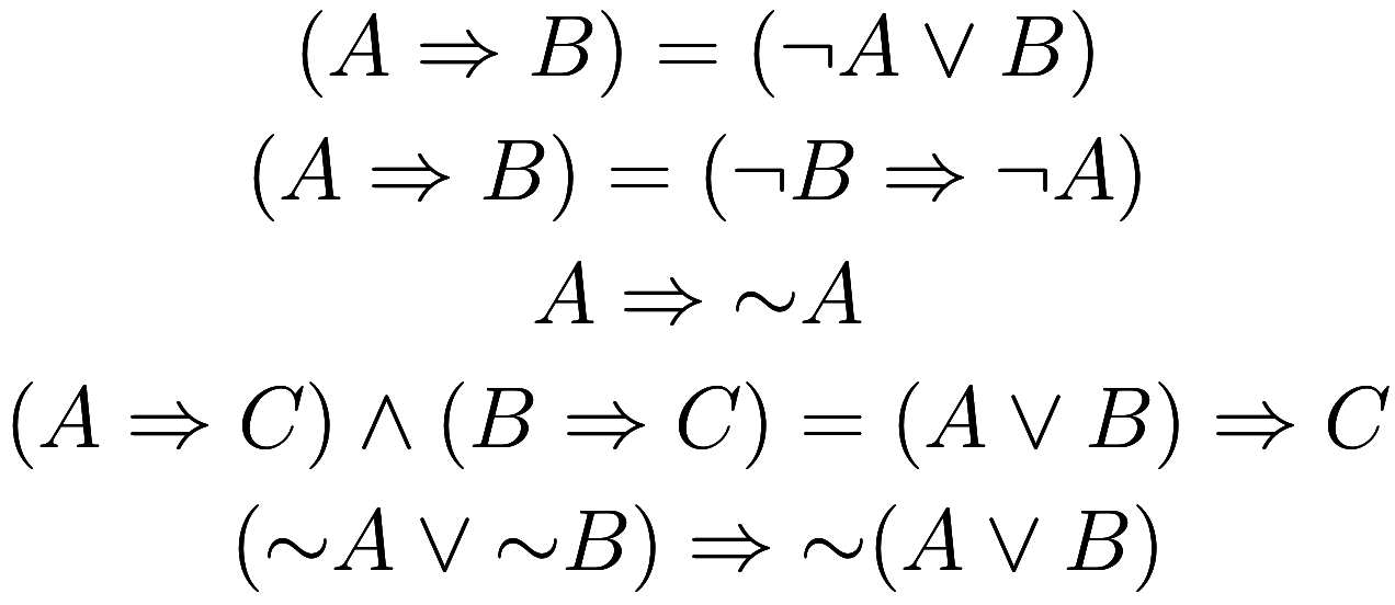
Note that the first statement above can be thought of us the definition of , the second is the contrapositive, and the third is one of the axioms of . Before we move on, let us prove the last two statements. To show the fourth statement, we have

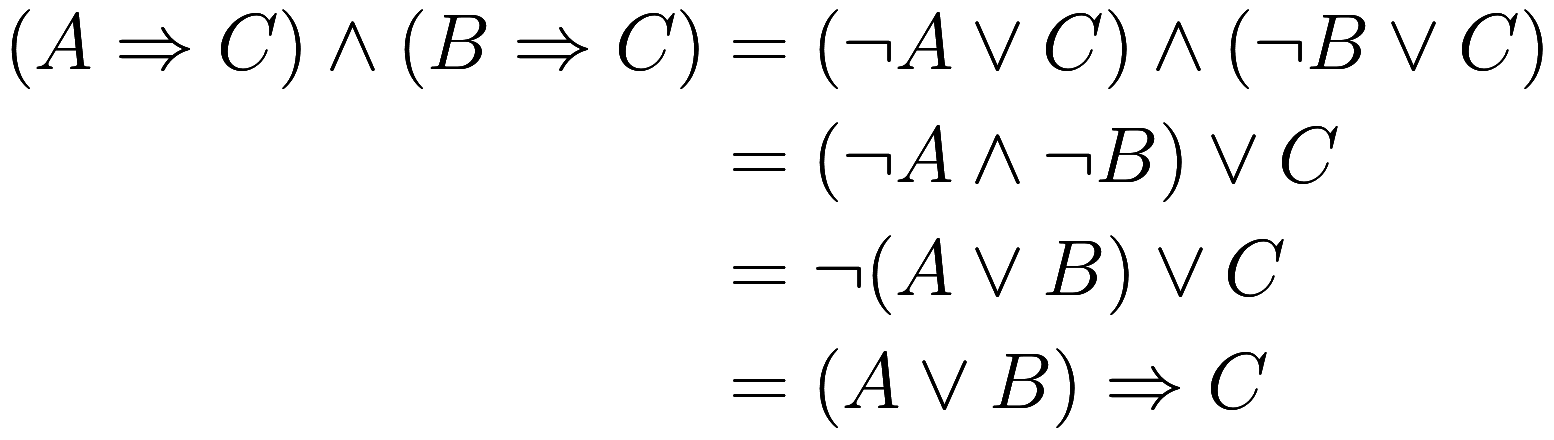
where we have used the definition of three times and basic properties of and .

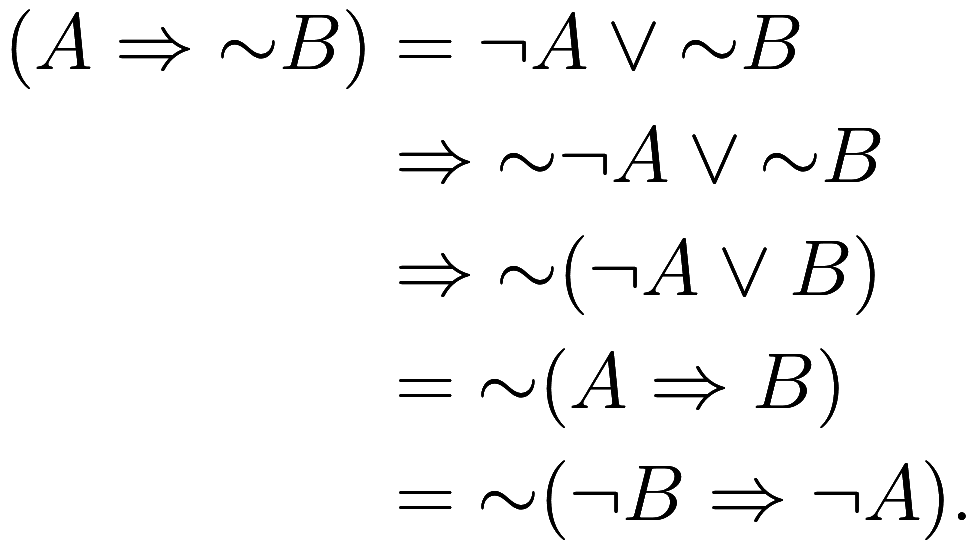
For the fifth statement, we have , and likewise , so by the fourth statement the conclusion follows. Note that the converse (i.e., flip the direction of ) is false: it is possible for to be probably-true, but neither nor is probably-true.

Let us return again to the contrapositive, which says that if then . We would like to use to make a similar statement, that if then . This is false (e.g., if and are true, but not nor , then the antecedent is true but the conclusion is false⁴You may recall that in ordinary logic we can test the validity of statements using truth-tables: that is, tabulate every combination of possible values of true and false for each variable, and then verify the claim simplifies to “true” for each combination. We could do something similar, but now each variable has three possible values: true, probably-true but false, and definitely false. Indeed this technique successfully disproved the statement here. However I am not sure this could be used in general, because of the existence of expressions like and and which cannot be simplified into depending only on the values of and .). However, a weaker form of the contrapositive is true: if , then . Let us prove that. First, since implies , therefore implies . Therefore

where we have used the various properties from the list of examples above.

How is this useful? Suppose we have some item whose truth is of interest, but we cannot directly observe . Instead has some consequence, , which is observable. If we observe , then we can conclude .

Of course the real world is rarely so generous as to have certainty, so rather than we only know the weaker consequence . Now from we cannot conclude , but we can probably conclude , as we have . This is not to be confused with definitely concluding , which would be .

This is exactly the formula used in hypothesis testing. We have some unobservable claim, , called the null hypothesis. To test , we build a statement of the form ; this process will be explained in more detail shortly. We then perform an experiment to measure . If we observe , then we can probably conclude : we reject the null hypothesis at some confidence level, representing a false negative rate.

We see from this the two main sources of confusion that arise in hypothesis testing. First, to make this deduction we must observe . If we observe then we can make no deduction (we “fail to reject the null hypothesis”), just as if and then we gain no information about . Second, even if we do observe , we do not conclude that is probably false; instead we probably conclude that is false. These sound very similar but this is the distinction between , which is true, and , which is false. It is common for people to mistakenly interpret the p-value as the probability that is true; but instead it is the probability of a false negative if is true.

Hypothesis testing

Time for the messy bit: how do we construct a statement of the form ? That is, we need to make a choice for . As an example, suppose we pick a random number from 0 to 1, and say that is the observation that the random number is bigger than 0.05. Then where means “with 95% confidence”. If we observe , that the random number is smaller than 0.05, we can reject at a 95% confidence level.⁵Obviously you should choose the desired confidence level for your application, and not blindly follow the traditional choice of 5% error rate, but for purpose of our discussion it is fine.

As an example, let us say that is the hypothesis that a certain population has a mean height of 2m and standard deviation of 0.1m. Using the choice for above, then is true where means 95% confidence. If we perform the experiment we either observe or . If the former, we deduce nothing; if the latter, we have at 95% confidence, which we express as “rejecting” the null hypothesis .

Obviously this is not a great choice of , as it has no relation to the underlying claim that we want to test. Our approach has a 5% false negative rate: there is a 5% chance of us rejecting even if it is true. We also have a 5% true negative rate, and have a 5% chance of correctly rejecting if it is false. Our goal then is two-fold: we want to choose a such that according to some desired false negative rate, and conditional on maintaining that false negative rate maximize the probability of observing if .

The task of choosing such a is usually broken up into 3 steps: choosing a test statistic, calculating a p-value, and choosing a false error rate (the threshold for the p-value). Frequently there is an obvious choice for that is the mathematically best way to distinguish the possibilities and , for a certain collection of observations; other times it is less obvious what the optimal choice is, or if there even is one, and we just have to pick something that seems good. Different choices for correspond to different statistical tests; one is not more correct than another, but one may have greater statistical power for the same significance threshold, and therefore be more likely to reach a useful conclusion for a given dataset.

Using again that is the claim that a population has a mean height of 2m and standard deviation of 0.1m, we will make a more sensible choice for . To have any chance of progress, we need observations that relate to in some way, so let us suppose we have access to a random sample of members of that population, and can measure their heights. Thus we have as data some collection of numbers representing these heights; these are random variables,⁶Formally a “random variable” means “a value randomly sampled from a probability distribution”. in that each time we perform the experiment we may get different values for the , and we suppose they are iid. Depending on our application, we might have much more complicated observations, including non-numerical data.

A test statistic is any real-valued function of the observations.⁷Well, technically that is the definition of a statistic. A test statistic is a statistic that is useful in hypothesis testing. Also it doesn’t really have to be real-valued; it just needs some ordering. We want to choose a test statistic that is informative about whether is true or false. In this case, the obviously best test statistic is the sample mean:

Next, we calculate a p-value. A test statistic is a random variable (because it is a function of random variables) and therefore follows some distribution. We want to choose our test statistic in such a way that if is true, we know the distribution the test statistic follows: in this case, is approximately normally distributed with mean 2m and standard deviation . The p-value is found by normalizing a test statistic to be uniformly distributed in the range 0 to 1, assuming is true. We do this by computing the cdf of the test statistic and applying it to the observed value of the test statistic; that is, we compute the percentile of the test statistic in its distribution. (We will discuss one-tailed vs two-tailed tests later.)

Finally, we choose a threshold such as 0.05, and is the observation that the p-value is greater than 0.05.

Thus, if is true, the p-value is a random variable uniformly distributed in the interval 0 to 1, and therefore there is a 95% chance of observing . That is, , from which we deduce , as desired: our test has a 5% false negative rate. However now we have improved on our previous choice of . If is false, the distribution of is not what we calculated above, and therefore the p-value is not uniformly distributed from 0 to 1. Hopefully the p-value strongly favors values below 0.05 – if so, we will have a high true negative rate (and so low false positive rate).⁸You are welcome to, say, suppose the population has a height mean of 1.5m and calculate the distribution of and under that assumption; if is large enough, the p-value will be strongly weighted towards 0.

While historically hypothesis testing was intended to give a reject/fail-to-reject binary outcome, as described above, in practice one usually reports p-values directly.

So far we have been staying close to propostional logic, with a bit of uncertainty mixed in. As we change course to look at Bayesian reasoning, we will fully accept the probabilistic nature of our computations. From now on we are using the letters , , …, to represent events, with the symbol to mean the probability of the event .

Bayesian reasoning

Suppose you have two exclusive events⁹In probability theory, an event is a statement which has a probability of being true. We assume events follow certain rules, such as if and are events then there is an event called , representing that both and are true, satisfying . and you wish to distinguish. Unfortunately we cannot observe them directly; instead we make some sequence of other observations .

If one of our observations were, say, incompatible with , then we would be done; by simple deductive reasoning we could say “ implies ; ; therefore ”. Instead each of our observations are consistent with either or – but, critically, not equally so. We measure the degree of consistency with the conditional probabilities¹⁰The symbol , read “(the conditional) probability of given ” is defined as the ratio . and . From this information it is a simple application of Bayes’ Theorem to compute , and repeated application to get .

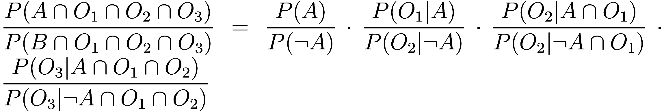
There is nothing deeper to performing Bayesian computation than repeated use of Bayes’ Theorem, but with a little organization we can gain better understanding of the process and be less likely to make mistakes. First, we can build a table of the information we know:

prior
observation 1
observation 2
observation 3

Because we will be interested in the event that all of the observations are jointly true , rather than only one or another of them being true, we have to use the probability of each observation conditioned on the previous ones also happening. If our observations are independent of each other then this is unnecessary, as in this case.

Next, let us use the definition of conditional probability:

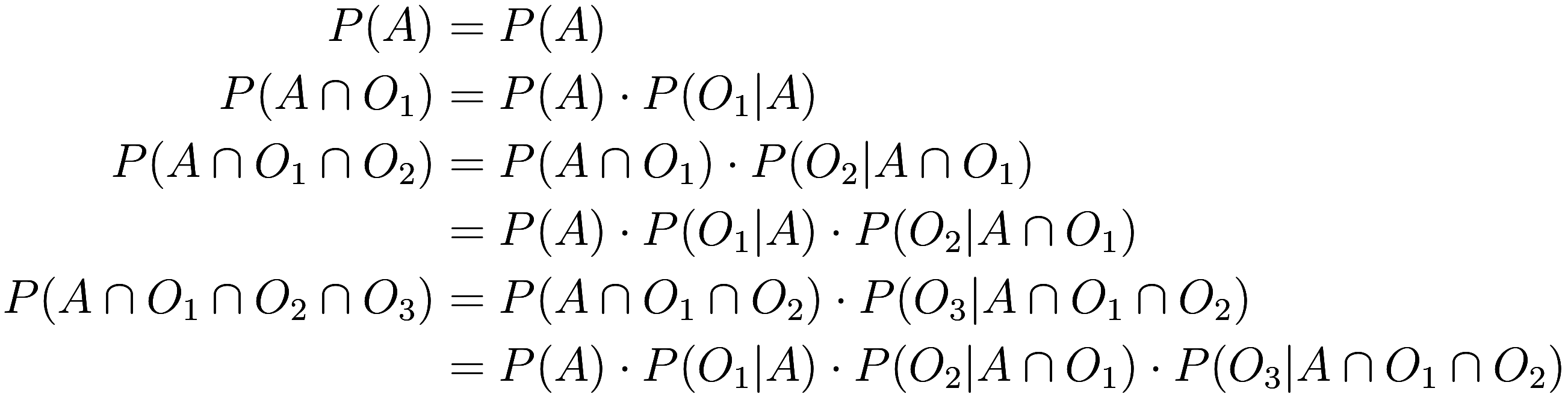
Thus, the cumulative products we get by just multiplying down the columns of the previous table are the joint probabilities:

-	1	1
prior
observation 1
observation 2
observation 3

(Note that mathematically there is nothing distinguishing the prior probability from any of our observations; the choice of what information to call “prior” versus “observation” is just a matter of convention. You can think of prior as the “null” or trivial observation: how much you should update your probabilities based on not making any observations at all.)

We should interpret each row as telling us the relative probability of either of the hypotheticals jointly with the cumulative observations. Initially, before making any observations, the prior probabilities and sum to 1 but as we apply successive observations the sum of each row will decrease and become smaller than 1. This residue probability (ie, the amount by which each row sums to less than 1) represents the chance of some hypothetical alternative in which at least one of the observations didn’t happen.

Ok, what good has this done us? Well, our goal is to find the conditional probability . This is just equal to the fraction of the th row that is in the first column:

Indeed, all that matters is the ratio of the two columns:

Since the columns of the second table were found by just multiplying the columns of the first table, the ratio of the columns of the second table are just the product of the ratio of the columns of the first table:

Thus we began with eight¹¹Actually seven, because we knew , so the first row only had one data point. pieces of data in the first table but it turns out that all we needed was four pieces of data, supposing we can directly measure these ratios.

Indeed frequently the ratio , called the Bayes factor, is easier to measure than either or separately; in messy, real-world scenarios the probability of the event might be wrapped up with many uncertain factors that have nothing to do with either or . Estimating requires assessing these irrelevant factors, but estimating the Bayes factor does not.

In extremes where probabilities get very close to 0 or 1 we can simplify matters further by taking logarithms everywhere – why multiply when instead you can add? We then have logarithmic Bayes factors where is the information contained in the first observation, with positive numbers informing us in favor of event , and negative numbers informing us against it. If the logarithm is base 2, then has units of bits. Adding up each of our pieces of information gives (Given a new piece of information , we can simply add it to the sum we have so far; this is called Bayesian updating.)

This result is also called the (conditional) log-odds of .¹²The log-odds of is defined as , but here we have conditioned on the observations . Log-odds can in some situations be more intuitive than ordinary probability, especially for extreme probabilities. A log-odds of 0 means a probability of 50%, and positive log-odds means an event that is more likely to happen than not. From the (conditional) log-odds of we can compute the ordinary (conditional) probability:

How does this work in practice? Suppose some event of interest has some probability of being true; start by computing the unconditional (ie, prior) log-odds of . We make a series of observations, and assess for each observation how much information it provides in favor of versus against it. We update our log-odds of by adding to it the information (positive or negative) from each observation. The result is the updated (ie, conditional on the observations) log-odds for . Alternatively, if we don’t want to work with logarithms, instead of adding up log-odds we can directly multiply probabilities.

Let us work an example. Suppose you are hiring an engineer, and you want to know their competency at a particular skill. You make three independent observations: they did adequately on an interview assessing that skill, they have an obscure certificate for that skill, and they went to University of Example which has a good engineering program. Most candidates, whether competent or not, do not have that certificate nor went to that university, so it is hard to assess the probability of those observations; but the relative probabilities, or Bayes factors, are easier to guess at. We have

			Bayes	log-odds
prior	0.1	0.9	0.111	-2.2
interview	0.4	0.1	4	1.39
certificate	-	-	1.2	0.18
UoE grad	-	-	2	0.69
total	-	-	1.0667	0.065

Adding up the last column we get a log-odds of 0.065, or a probability of 51.6%, just barely above even odds that the candidate has this particular skill.

This example also illustrates a second important principle to understand with Bayesian reasoning: it can applied to any situation, and always gives an answer, regardless of how appropriate the technique is for the application. I certainly hope no one involved in hiring candidates is using a calculation of this nature to help make that decision, or at least not with the same lack of care as I did above. One must pay close attention to potential problems: did you account for all the available evidence? how accurate are your probabilities? how robust is your result to changes in the data? The messier and more “real-world” your situation, the easier it is to run afoul.

How do Bayesian reasoning and hypothesis testing relate?

The short answer is very simple: the conditional probability of making an observation conditional on the null hypothesis is the p-value of that observation.¹³Following a conversation with Michael Weissman in which he disagreed with this statement, I should clarify that this is only for a binary observation. More generally one should say that the conditional probability is related to the p-value, with the nature of that relationship depending on the definitions chosen for a particular application.

In Bayesian reasoning we start with a prior probability , a conditional probability , and the complementary pieces of information ¹⁴Which of course is redundant with , since and , and use these to compute an update:

In hypothesis testing, the only piece of data we have is the p-value . We can’t compute because we don’t have the other required pieces of data.

If we have all three pieces of information then it makes sense to go ahead and compute the updated probability ; however if we do not have access to those last two numbers, or their accuracy is very low, it can be more useful to directly report a p-value and not attempt to compute .

In primary scientific research, those two numbers are often inaccessible due to two features of the null hypothesis: the null hypothesis being non-probabilistic, and being very narrow or asymmetric.

Suppose is a statement like “it will rain tomorrow”, and we want to estimate the probability of tomorrow’s weather based on observing today’s weather. It makes a lot of sense to start with a prior probability (based on historic rainfall frequency) and update it appopriately. But if is a statement like “neutrinos are massless” or “fracking does not influence earthquakes” then it is not meaningful to speak of probabilities like or .¹⁵Note that is still meaningful, so long as the observation is probabilistic in nature. We could interpret to mean our level of confidence in , i.e., as information content, but this often has more to do with the mental state of the researcher than with .

Second, Bayes theorem is fully symmetric between and , but frequently in scientific research these hypotheses are not symmetric. The classic example is testing if a coin is fair: suppose we observe 30 heads in 100 coin flips (iid), and we want to test the null hypothesis that the coin is fair. Here is a very narrow and specific claim that lets us easily compute a p-value . The negative is unspecific: the coin has some bias, but it could be any nonzero amount. The probability depends on how biased the coin is, so we need additional information like a probability distribution for the amount of bias. This is a lot to ask for when we don’t even know if the coin is biased at all!

Finally, even if we had this extra data and could compute , frequently that is less useful than reporting raw p-values. Suppose you are doing secondary research, and want to estimate ; you find that primary research into the effects of has identified a series of unrelated observations that give information about . Each of these observations has been made by different research teams with different specialities. If each team reported their own estimate for , it would be a troublesome and error-prone process to combine these estimates into a single value for : each team will have a different estimate for with different assumptions; each team would incorporate different evidence (perhaps the researchers investigating the phenomenon were unaware of the existence of and omitted it entirely; or the researchers incorporated some other evidence that was later found to be unreliable). For you to compute would require first undoing all the computations that each team did to reconstruct the underlying p-values ; much simpler if they just reported these p-values directly.

The reason primary researchers report p-values is that this is usually the natural end point of their research; synthesizing the p-values of many different observations into a single posterior probability is the job of secondary research. Each probability might involve a completely different physical process and speciality, so it is most suitable to have each term investigated separately by experts in the appropriate field.

(Todo; might add some explanatory text on how to convert between bayes factors and p-values)

Appendix: one-tailed vs two-tailed tests, and other messiness

Recall from the first section that the hypothesis testing method involves three steps:

1. Compute a test statistic, which is a random variable that is a function of some collection of observations.
2. Normalize the test statistic so that it is uniformly distributed in the range [0, 1]. This normalized value is called the p-value.
3. Choose a desired false negative rate, and “reject” the null hypothesis if the p-value is below this threshold.

We slightly glossed over the second step, giving one way to normalize the test statistic by applying its cdf.

Choosing the normalization method is every bit as important as choosing the test statistic (though usually obvious once the test statistic has been chosen); as with the choice of test statistic, any choice is valid so long as the result is uniformly distributed in the range [0, 1], but not every choice might have the same statistical power (i.e., false positive rate).

Recall that we want the p-value to be as low as possible when conditioned on ; this maximizes the chance of a correct rejection of , since we reject when the p-value is below the threshold. Therefore when normalizing, we first sort all possible values of the test statistic by how likely they are under the condition of . Thus, the most likely outcomes will have the lowest p-values.

Slightly more carefully, what we are sorting by is how informative each possible value is in favor of over ; that is, we are sorting by the Bayes factors .

For example, suppose our null hypothesis is that a coin is fair, and we observe that the coin had 30 heads out of 100 flips. Our test statistic is the number of heads, which when conditioned on is approximately normally distributed with a mean of 50 and standard deviation of 5. We can normalize a normal distribution into a uniform distribution by applying the cdf; then 0 heads gives a p-value of 0, 50 heads gives a p-value of 0.5, and 100 heads gives a p-value of 1. What is the p-value of 30 heads? This is 4 standard deviations below the mean, which we can look up in a standard normal table is a percentile of 0.00003; that is our p-value, and we can feel confident in rejecting the null hypothesis that the coin is fair.

While this worked okay, depending on the application this was not the best choice of normalization. If instead we observe 70 heads out of 100, we would have gotten a p-value of 0.99997, and we would fail to reject the null hypothesis even though we know intuitively that the observation contains enough information to do so. We would have done better if we had sorted the possible observations by how informative they are in rejecting the null hypothesis. Here finding 0 or 100 heads is the most informative, so they get the lowest p-values, followed by 1 or 99 heads, then 2 or 98 heads, and so on, ending with 50 heads getting assigned a p-value of 1. As before, this is done so that the result is uniformly distributed in the range 0 to 100. Now if we observe 70 heads, this has a higher p-value than any observation of 0 to 29 or 71 to 100 heads, but a lower p-value than 31 to 69 heads; therefore it gets a p-value of 0.00006,¹⁶The total probability of seeing 0 to 29 or 71 to 100 heads, conditioned on , is 0.00006. again comfortably rejecting the null hypothesis that the coin is fair.

As we are sorting the observations by their Bayes factors , this sorting depends on the choice of alternate hypothesis . If is that the coin has any nonzero bias, then the sorting method we just used is appropriate, and is called a two-tailed test; but if is more specifically that the coin is biased in favor of tails, then the observation of 70 heads out of 100 does not significantly favor either the null or alternative hypotheses, and so gets the p-value of 0.99997 we had originally calculated. This is the one-tailed test. For example, when testing a cancer medication in rats, our null hypothesis is that it has no effect, and our alternate is that it reduces cancer rate, so a one-tailed test is appropriate in that we would not draw any conclusions from an observation of it increasing cancer rates.¹⁷And also in that rats, unlike certain biased coins, have one tail. This was an actual question I got from a cancer researcher who knew how to perform the calculations for a one-tailed and two-tailed t-test but not which one was appropriate, and only one of the results was “significant”.¹⁸Apparently the group’s statistician was on vacation at the time; why the researcher thought to ask a 19-year old kid from a foreign country is unclear. Probably the better answer would have been that the magical 5% confidence threshold is arbitrary and no great import should be assigned to whether your results fall above or below that line.

(A little subtlety: how do we sort by the Bayes factors if we can’t compute them without choosing a specific bias for ? For the one-tailed coin test, it does not matter; the sorting is the same for any possible bias even though the actual values are not. For two-tailed, we have to assume that bias in favor of heads is equally likely as bias in favor of tails, and maybe some further assumptions.)

While frequently choosing how to normalize the test statistic amounts to simply choosing between a one-tailed or two-tailed test, in principle it could be any possible normalization scheme: maybe the two tails could be weighted differently, or the sorting goes from inside out, or even numbers come before odd numbers, etc etc. The test statistic doesn’t even have to be a number – all that is required is that it can be sorted by the Bayes factors.

(Addendum. I couldn’t find a decent splash image for this post online, so I asked a bot to draw a picture of “hypothesis testing” and ended up with this mess.)

Follow RSS/Atom feed for updates.