With the US Senate and electoral college heavily biased against states with larger populations, there sometimes arises the misconception that the apportionment of seats in the US House of Representatives is similarly biased. A brief glance at the number of people in each district for every state shows that there is no such significant bias for or against larger states. (Later, we will consider the matter in more detail and explore the tiny biases that do exist.)
We leave aside questions such as US citizens who have no voting representation in Congress, how districts are drawn within each state, and how the population of the states is determined, and only examine how many seats in the House each state is allocated.
A brief overview of US Congressional apportionment and its history
can be found in this
CRS report. Since 1941, the fixed number of seats in the House has
been apportioned amongst the states after each decadal census according
to the Hill method of apportionment. Let be the population of the
th state, and for positive integers
define
![]()
Then the Hill method apportions seats by taking the
largest of the
, with state
gaining one seat for each
so taken. As law requires that each
state is allocated at least one seat, we require that the
are all taken before any
with
.
Equivalently, if is the number of seats allocated to state
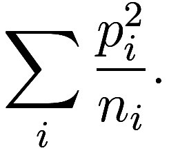
, then the Hill method minimizes

Let be the total population. Then this is equivalent
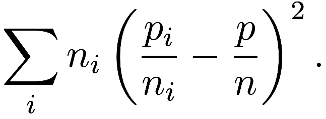
to minimizing

The quantity is sometimes called the ideal district
size; it equals the population-weighted harmonic mean of the
district sizes
, which in general is not equal to
the arithmetic mean of the district sizes.
Define the voting power of each person to be the number of
House seats their state has, divided by the population of the state;
each person in state has the same voting power
, which is the reciprocal of
the district size within that state. The average person’s voting power
is
, and so does not depend of the choice
of apportionment. In the US after 2010,
![]() , corresponding to an ideal district
size of
, corresponding to an ideal district
size of people.
We consider the 2010 House apportionment, and are interested in
whether a person’s voting power depends in some way on the size
of their state. A simple test is to do a linear
regression of
against the independent variable
; while there are
![]() data points, each person in the same state has
the same data, so we can simply do a weighted linear regression on 50
data points.
data points, each person in the same state has
the same data, so we can simply do a weighted linear regression on 50
data points.
However, almost all of the variation in voting power occurs in the
smallest states, which are most subject to the restriction that each
state has an integer number of seats. The state with the lowest voting
power is Montana, having 1 seat for 994416 people and thus voting power. The next larger
state is Rhode Island, having 2 seats for 1055247 people and thus
![]() voting power, the largest of any state and
88% more than Montana.
voting power, the largest of any state and
88% more than Montana.
A linear regression might pick up on these significant variations
amongst the small states, but when we speak of bias in House
apportionment we are often most interested in the small states
collectively compared to the large states collectively. To measure this,
we sort the people by the size of the state they are in, and group
together those in the first half as the “small state” sample and those
in the second half as the “large state” sample. (The median person is in
Georgia, which will thus lie partially in the small states and partially
in the large states.) Then we find the difference in the average voting
power of the people in these two samples: this equals the difference in
number of seats those states received, divided by .
The results can be seen in the figure:
2010 US House apportionment. For each state, we plot its population
and voting power
. The black line shows the average
voting power
. In green is the average voting power
within the small states and within the large states. In red is a linear
regression of voting power against population.
The large states have an average voting power larger than the small states,
an improvement of about 0.9%; we call this difference the voting
power gap. The slope
![]() of the regression line is in
units of voting power per person (that is, per person squared), so we
must multiply by a population to make it the same units as the voting
power gap. We will find that multiplying by the population of New York,
19421055, makes a good comparison with the voting power gap, so the
scaled voting power slope is
of the regression line is in
units of voting power per person (that is, per person squared), so we
must multiply by a population to make it the same units as the voting
power gap. We will find that multiplying by the population of New York,
19421055, makes a good comparison with the voting power gap, so the
scaled voting power slope is ![]() .
.
Thus we see that, by either measure of bias that we investigated, the 2010 apportionment is biased a very small amount in favor of large states.
Of course, if the House had only 50 seats, then each state would have one seat, and it would be massively biased in favor of small states. Clearly for small number of seats a bias exists, and for 435 seats it appears to be insignificant. We investigate how the voting power bias changes as the number of seats in the House changes.
Voting power gap (green) and scaled voting power slope (red, scaled by the population of New York) with the Hill method of apportionment for each number of seats from 50 to 600.
We see that the two measurements of voting power bias substantially
agree with each other, up to a constant scaling factor. While there is
quite significant bias for small states when the number of seats in the
House is small, this rapidly decreases with increasing numbers of seats.
While it happens that the 2010 census data apportioned with 435 seats
favors large states very slightly over small states, this is a bit of an
anomaly, as the Hill method tends to favor small states slightly.
Looking at seat numbers from 400 to 500, we see that at these sizes with
the 2010 census data there is typically a voting power bias of about
in favor of small states, which is a bit
less than 1% of average voting power.
This is an advantage of one seat for every 100 million people, which put into absolute terms is about 1.5 seats. As the number of seats is increased further into the thousands and beyond, there continues to be a slight but diminishing bias in favor of small states. As the number of seats increases, the total voting power of all people increases, while the voting power gap decreases, and thus the proportional bias relative to total voting power decreases quite rapidly. That is, even as the number of seats increases, the difference in how many of those seats go to small states or large states decreases.
In part 2, we will consider other apportionment methods and their theoretical properties.
Follow RSS/Atom feed for updates.