Why is it warmer in summer?

2022 September 13

It’s not a trick question: yes, it is warmer in summer because there is more sunlight. But there is surprising nuance in trying to nail down exactly what is going on – and if you don’t believe me, which of the following explanations sounds more plausible?

The Earth warms during the day and cools during the night¹Via radiation of infrared light to space due to the blackbody effect; see my series on the greenhouse effect for more details.; summer days are longer and therefore able to reacher a higher temperature.
The Earth warms during the day and cools during the night; on long days, warming exceeds cooling, so as summer carries on the Earth accumulates more and more heat.

These are very different theories – if, say, an Earth year were only 20 days long (and each day were still the same length), the second explanation predicts very mild seasonal variation, while the first predicts that seasonal variation would be unchanged.

We can see right away that the first explanation is not fully correct. Consider a location that is 45 degrees from the equator, such as Milan. The longest day of the year is the summer solstice, on June 21:

Length of day in Milan, Italy. © WeatherSpark.com

However, the hottest day of the year is more than a month later:

Average temperature highs and lows in Milan, Italy. © WeatherSpark.com

So after the solstice, the days are getting shorter, but Milan keeps getting hotter. Perhaps the second explanation is correct, then. Can we delve in and test it further?

Theoretical model

We are interested in a fixed location on Earth, and let us suppose that it has a temperature, or more precisely heat energy²We suppose that the heat capacity is constant over the range of temperatures of interest, so energy and temperature are linearly related., of $E$ , varying with time $t$ . Sunlight warms the Earth, and infrared emissions cool it; the latter is approximately proportional to $E$ ³Black-body radiation varies with the fourth power of temperature per the Stefan-Boltzmann law, so we need a cubic correction factor, which is modest over the range of temperatures over interest; but we are not trying to be quantitative yet.. Then the governing equation for $E$ is

$\frac {dE}{dt} = \omega (S - E)$

where $S$ represents insolation, which may depend on $t$ , and the various constants are absorbed into $\omega$ which has units of one over time. $\omega$ is a frequency, and $1 / \omega$ is the characteristic timescale for the Earth system to restore equilibrium.

$S$ has units of temperature (or energy, according to the units chosen for $E$ ) and represents the equilibrium temperature of that location of Earth. If $S$ were constant, then the temperature $E$ would simply exponentially decay to $S$ . However let us now take $S$ to be the day-averaged insolation at 45 degrees, which is well-approximated by a sine wave:

$S = S_0 + a \cos (\tau t / P)$

where $\tau = 2\pi$ and $P$ is the insolation period, i.e. 1 year. So we need to solve

$\frac {dE}{dt} = \omega (S_0 + a \cos (\tau t / P) - E).$

Theoretical day-averaged insolation at top of atmosphere as a function of latitude \phi and time of year \theta, chosen so that \theta = 0 is the spring equinox for the hemisphere with \phi > 0. The black regions are polar nights. Peak day-averaged insolation occurs at the poles at the height of summer, receiving a theoretical 550 Watts per square meter. However, note that the tropics receive both higher instantaneous insolation (at local noon) and higher year-averaged insolation. In the mid-latitudes, insolation is approximately sinusoidal. More information here. — Theoretical day-averaged insolation at top of atmosphere as a function of latitude $\phi$ and time of year $\theta$ , chosen so that $\theta = 0$ is the spring equinox for the hemisphere with $\phi > 0$ . The black regions are polar nights. Peak day-averaged insolation occurs at the poles at the height of summer, receiving a theoretical 550 Watts per square meter. However, note that the tropics receive both higher instantaneous insolation (at local noon) and higher year-averaged insolation. In the mid-latitudes, insolation is approximately sinusoidal. More information here.

A pretty sensible (and correct, fortunately) guess is that $E$ is also a sine wave, with $E = S_0 + A \cos (\tau (t - t_0) / P)$ . Here, $t_0$ indicates the phase offset between peak insolation and peak temperature: for Milan, we had $t_0 = 35$ days.

We could thus solve for $E$ very directly, referring to some less-used trig identities for sums of sines. However, the easiest derivations for these identities are from complex numbers, so instead we will forestall needing trig at all by using complex numbers from the start. First, notice that the differential equation for $E$ is linear: if $E_1, E_2$ are the temperature functions corresponding to the insolations $S_1, S_2$ , then

$\frac {d(E_1 + E_2)}{dt} = \frac {dE_1}{dt} + \frac {dE_2}{dt} = \omega ((S_1 + S_2) - (E_1 - E_2))$

and thus $E_1 + E_2$ is solution for an insolation of $S_1 + S_2$ .⁴Indeed this linearity is how we knew that the constant term of $E$ is $S_0$ . In particular, if $S$ is complex, the real and imaginary parts act independently of each other. Therefore, instead of the previous choice for $S$ we can use

$S = S_0 + a e^{it / P}$

and we plug in $E = S_0 + A \exp(\tau i (t - t_0) / P)$ in the differential equation to get

$\begin{aligned} A (\tau i / P) e^{\tau i (t - t_0) / P} &= \omega a e^{\tau it / P} - \omega A e^{\tau i (t - t_0) / P} \\ A ((\tau i / P) + \omega) &= \omega a e^{\tau it_0 / P} \\ A ...$

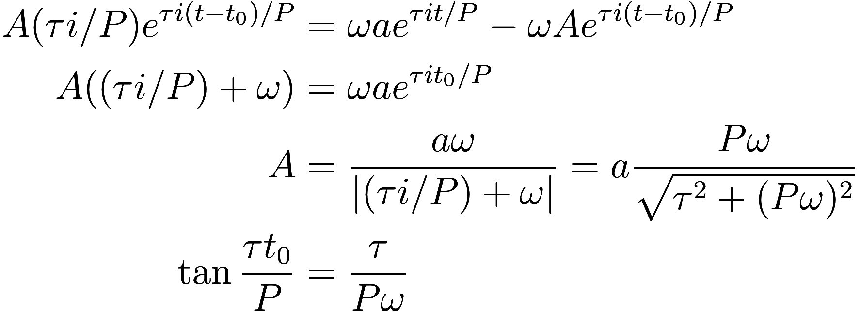
Then, returning to real numbers, we get that the solution to the differential equation is

$E = S_0 + \frac {P\omega}{\sqrt{\tau^2 + (P\omega)^2}} a \cos(\tau (t / P) - \arctan (\tau / P\omega)).$

Here $P\omega$ is a unitless number representing how many “times” the system can relax to equilibrium within one period $P$ of the forcing. When it is very large, the system rapidly approaches equilibrium: the amplitude $A$ is close to the forcing amplitude $a$ , and the phase shift $\tau t_0 / P$ is nearly zero. When $P\omega$ is quite small, the system takes many times the length of a single forcing period to reach equilibrium, thus greatly damping the amplitude $A$ , and causing the phase shift $2\pi t / P$ to approach a maximum of 90 degrees (i.e., 3 months out of phase).

Thus, the differential equation for $E$ is essentially a low-pass filter: components of $S$ with a frequency higher than $\omega$ are dampened, whereas components with a lower frequency are passed through. In fact, it is exactly the equation for an RC circuit with $1 / \omega = RC$ .

How can we make use of this solution? We will not be able to sensibly predict $\omega$ from first principles as it depends on a wide variety of physical attributes of the terrain and atmosphere, such as heat capacities, thermal conductivity, albedo, emissivity, etc. Therefore we cannot predict $S$ , or $a$ , either: while insolation in units of Watts per square meter can be observed easily, we have folded an unknown constant into $\omega$ to bring $S$ to units of temperature. Thus the amplitude $A$ is not useful.

However, observation of $E$ does tell us the phase-offset $t_0$ , and therefore $\omega$ . In the case of Milan, where we observed $t_0 = 35$ days, we get $\tau / P\omega = \tan (\tau t_0 / P) = 0.867$ or $1 / \omega = 0.109P = 40$ days⁵ $\tan x \approx x$ for small $x$ so it is not a surprise that $1 / \omega$ is approximately equal to $t_0$ . Thus the timescale for temperatures in Milan to approach equilibrium is (in theory!) 40 days.

With the time to restore equilibrium so much longer than a single day, and comparable to the length of a season, this supports our second explanation, that summers are hot because of the accumulation of heat locally over an extended time.

Replicating diurnal and seasonal cycles

But there is a critical flaw in this argument so far! To get here, we used the daily-averaged insolation $S$ – we let sunlight smoothly vary over the seasons, completely erasing the existence of day and night. And, consequently, the resulting temperature $E$ also smoothly varies with the seasons, and does not accurately replicate the observed day-night cycle of hot and cold.

To better understand this issue, let us crudely approximate the diurnal plus seasonal cycle as a sum of two sine waves. As the differential equation for $E$ is linear, the solution will be

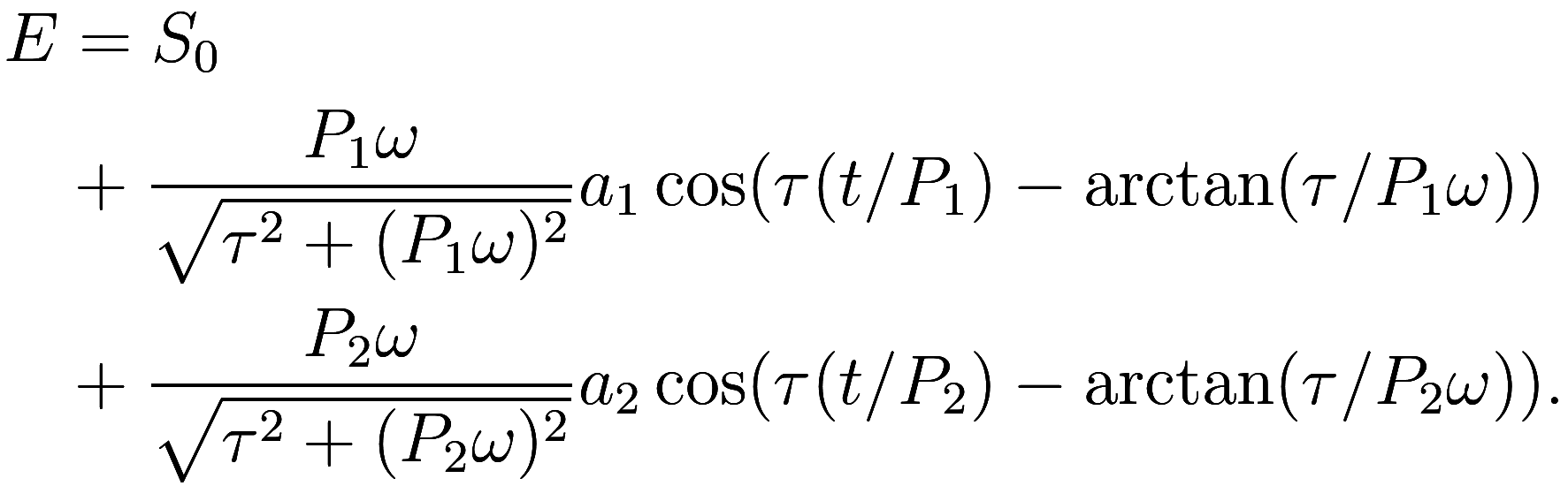
$\begin{aligned} E &= S_0 \\ &+ \frac {P_1\omega}{\sqrt{\tau^2 + (P_1\omega)^2}} a_1 \cos(\tau (t / P_1) - \arctan (\tau / P_1\omega)) \\ &+ \frac {P_2\omega}{\sqrt{\tau^2 + (P_2\omega)...$

(More generally, we could use this technique to find the solution for any periodic forcing function by taking the Fourier transform to decompose it into a sum of sine waves, solve them separately, and take the sum of the solutions.)

Here, there are two periods: $P_1$ , say, is one day, and $P_2$ is one year. The resulting temperature function also varies with these two periods. And indeed, we observe that temperatures vary throughout the day, and throughout the year.

So, have we fully explained observed temperature variations? Not quite, we have two problems, with the phase offsets and the relative amplitudes. As we saw above, we expect $1 / \omega$ to be on the order of 40 days to be able to produce the observed phase offset of the annual temperature cycle. However $1 / \omega$ is then 40 times larger than $P_1$ , so the phase offset of the diurnal temperature cycle will be 90 degrees (a quarter phase).

Phase offset of diurnal cycle

What is the observed phase offset of the diurnal temperature cycle? Well, sunlight does not actually act like a sine wave over the course of a day: it is more of a truncated sine wave, as solar heating does not become increasingly negative as the night gets deeper – once sunlight goes to zero it goes no lower.

In the $P_1 \ll 1 / \omega$ regime, the morning low and evening high are predicted to occur at the point where solar heating is equal to its average daily value; this is a generalization of the quarter phase offset from sinusoidal forcing to arbitrary periodic forcing.

Ignoring atmospheric phenomena, solar heating during the day is proportional to the cosine of the solar zenith angle, i.e., the angle between the sun and straight up, and is given by

$\cos \Theta = \sin \phi \sin \delta + \cos \phi \cos \delta \cos (\tau t / P_1)$

where $\Theta$ is solar zenith angle, $\phi$ is latitude, $\delta$ is declination of the sun⁶the angle between the subsolar point and the equator, and $t$ is time of day, with $t = 0$ being solar noon and $t = P_1 / 2$ being solar midnight.

The intensity of sunlight varies with its angle $\Theta$ , being most intense when bearing directly down; specifically, the intensity is proportional to $\cos \Theta$ . When $\cos \Theta > 0$ corresponds to exactly when the sun is above the horizon.

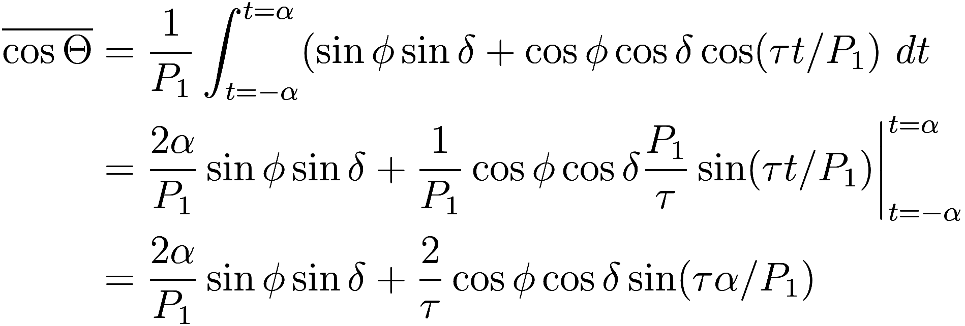
Thus we wish to find the average positive value of $\cos \Theta$ as $t$ varies, and so need to identify the time of sunrise and sunset (when $\cos \Theta = 0$ ). Sunrise and sunset occur at $t = \pm \alpha$ where

$\cos \frac {\tau \alpha}{P_1} = -\tan \phi \tan \delta.$

Then the average daily solar heating is

$\begin{aligned} \overline{\cos \Theta} &= \frac 1{P_1} \int_{t = -\alpha}^{t = \alpha} (\sin \phi \sin \delta + \cos \phi \cos \delta \cos(\tau t / P_1)\ dt \\ &= \frac {2\alpha}{P_1} \sin...$

Now we need to solve for $\cos \Theta_m = \overline{\cos \Theta}$ to find the angle $\Theta_m$ of the sun at which point it is providing the mean solar heating; this will occur at the time $t_m$ which is predicted to be the the temperature lows / highs. We have

$\cos (\tau t_m / P_1) = \left(\frac {2\alpha}{P_1} - 1 \right) \tan \phi \tan \delta + \frac 2 \tau \sin(\tau \alpha / P_1)$

Let us assemble a few example values. First, we tabulate sunset times $\alpha$ , listed in hours after solar noon:

	equinox	summer solstice	winter solstice
equator	6	6	6
30 degrees	6	6.97	5.03
45 degrees	6	7.71	4.29
60 degrees	6	9.24	2.76

Then, the predicted time $t_m$ of the daily temperature maximum, again in hours after solar noon:

	equinox	summer solstice	winter solstice
equator	4.76	4.76	4.76
30 degrees	4.76	5.22	4.20
45 degrees	4.76	5.49	3.70
60 degrees	4.76	5.86	2.53

Again let us consider Milan, which sits at 45 degrees of latitude. How do these predictions fare?

Solar midnight, sunrise, noon, and sunset in Milan, Italy. © WeatherSpark.com

Temperature variation with time of day in Milan, Italy. © WeatherSpark.com

For most of summer, solar noon is around 1.30pm local time. At the solstice, solar noon is 1.25pm, and the peak temperature is historically observed at 4.30pm, 3 hours later. This is noticeably earlier than predicted peak temperature. Worse yet, the temperature minimum is at 6am, just a few minutes after dawn! This is about 7.5 hours before solar noon, again much earlier than the prediction.

The prediction is even worse at the winter solstice. Local noon is at 12.21pm, sunset 4.42pm, and sunrise 8am. The predicted temperature maximum and minimum are at 4.03pm and 8.39am, but are observed at 2.30pm and 6.45am. In particular, temperatures are already rising (very slightly) before sunrise, whereas we should have expected temperature to linearly decline through the whole night, as the Earth is shedding heat to space at a uniform rate.

This does not just occur in Milan; for almost any location in the world, the actual phase offset for the diurnal temperature cycle is much lower than the predicted phase offset. Furthermore, the observed diurnal temperature cycle tends to be quite asymmetric, with the daily low around dawn and the daily high a few hours after noon, despite the solar forcing being approximately symmetric.

Relative amplitudes of diurnal and seasonal variations

Now let us consider the second problem: the relative amplitude of the diurnal and seasonal variations.

When we were considering only a single cycle, the amplitude was not helpful to consider because of the unknown constants involved; but with two variations at different periods (one daily and one yearly), we can compare their relative amplitudes and see if it is consistent with observations.

As our differential equation for $E$ is a low-pass filter, variations of higher frequency than $\omega$ will have their amplitude scaled downwards proportionally: when $P_1 \ll 1 / \omega$ , we have

$A_1 = \frac {P_1\omega}{\sqrt{\tau^2 + (P_1\omega)^2}} a_1 \approx \frac {P_1\omega}{\sqrt{\tau^2}} = \frac {P_1\omega}{\tau} a_1$

whereas for $P_2 \gg 1 / \omega$ we have

$A_2 = \frac {P_2\omega}{\sqrt{\tau^2 + (P_2\omega)^2}} a_2 \approx a_2.$

Recall that our observations in Milan suggest the timescale $1 / \omega$ is approximately 40 days, giving us

$\begin{aligned} A_1 &= 0.00398 a_1 \\ A_2 &= 0.824 a_2 \end{aligned}$

Thus the amplitude of the diurnal cycle in Milan should be supressed 207 times more so than the seasonal cycle. The difference between the high and low temperature in Milan is typically around 10 C, whereas the difference between summer and winter temperatures is about 20 C, so observations give $A_2$ is about double $A_1$ . To produce these observations, then, the diurnal variation $a_1$ in insolation needs to be 100 times greater than the seasonal variation $a_2$ .

The solar heating during the day is $\cos \Theta$ times the solar constant, which on solar noon at the summer solstice at 45 N is

$\cos \Theta = \sin \phi \sin \delta + \cos \phi \cos \delta = 0.93$

and at solar midnight is zero, for a daily range of 0.93⁷The diurnal cycle in solar heating is only poorly approximated by a sine wave; the “effective” daily range should be somewhat larger, but not enough so to change any conclusions.. The daily range at the winter solstice is even less, being only 0.368 at solar noon and 0 at solar midnight.

For the seasonal variation, we compare the daily averaged solar heating $\overline {\cos \Theta}$ at the two solstices. In summer we find 0.367, and in winter 0.0858, for a range of 0.281.

Thus the amplitude of the diurnal variation in forcing is up to around 4 times larger than the amplitude of the seasonal variation, but we needed an amplitude 100 times larger to replicate the observations.

The specific numbers will vary quite a bit from location to location, especially the diurnal and seasonal variations in temperature, which strongly depend on the complex behavior of local climatological conditions. None-the-less we would consistently find that our predictions from this model substantially understimate observed diurnal temperature swings: if it really needs most of a season for local temperatures to reflect changes in solar forcing, then individual days and night would be substantially smoothed over.

Reality

We are left with an irreconciliable conflict: we can explain the seasonal lag in temperatures by supposing that a location is gradually warmed over the course of season, or we can explain the diurnal lag in temperatures by supposing that a location is gradually warmed over the course of a day, but we cannot do both with a single physical object with a single response timescale. Either it responds on a timescale comparable to a day, in which case there would be no seasonal lag, or it responds on a timescale of a season, in which case its diurnal lag is much too large and diurnal variation much too small.

Clearly the differential equation for local temperature $E$ does not accurately reflect the actual processes going on that determine the temperature at a location; let us consider more carefully what is going on. Our first question should be, what does the temperature “at a location” on Earth mean – what is the actual physical object being measured? The graphs shown above reflect measurements of air temperature, but air is not particularly stable, and certainly does not stick around for multiple seasons. Worse yet, air near the surface receives very little direct solar heating: it is mostly heated by the Earth below, and to a lesser extent by air above it, and half of the heat it radiates goes down into the Earth instead of out towards space.

Perhaps more useful is the temperature of the solid Earth itself. This is directly heated by the sun – at least, the very top of it is. (Well, on much of the Earth it is the vegetation on top of the ground that is heated by the sun, which in turn mostly loses heat to the surrounding air and not into the ground.) We now have the problem of asking how deep into the Earth we should be considering: further under the surface temperatures are smoothed out on a longer time scale. The diurnal cycle of temperature only occurs in the top 10 to 20 cm, and the seasonal cycle is completely smoothed out at depths below 10 to 20 m.

Seasonal cycle in underground temperatures at various depths. Notice that at greater depth, variations are suppressed, as well as lagged. Source of data is unclear, possibly observations in Virginia.

What’s more, temperatures at depth are lagged relative to the surface, so that around perhaps 5 meters ground temperature is often hottest in winter⁸Note that the differential equation we’ve been using so far can only produce a phase shift of up to a quarter phase. The reason that temperatures underground can be phase shifted by more than that is that they do not directly interact with the surface, but rather interact via soil at an intermediate depth. Each “layer” of soil is slightly phase shifted and slightly damped relative to the layer above it, so these phase shifts can add up arbitrarily high at depth.. Temperatures many thousands of years into the past can be reconstructed by simply digging a deep enough borehole and measuring the temperature there.

All of this of course presumes we are talking about a location on land: in the ocean the concerns are different but no easier, with issues of how deep sunlight can penetrate into the water and ocean currents, particularly coastal upwelling.

A simple improvement over the differential equation above is the approach of Cronin and Emanuel (2013). They consider the temperature anomalies $T_S'$ of the surface and $T_A'$ of the air just above the surface, and assume (their equation 1)

$\begin{aligned} C_A T_A' &= \lambda (T_S' - T_A') - B T_A' \\ C_S T_S' &= \lambda (T_A' - T_S') \end{aligned}$

where $C_A, C_S$ are the heat capacities of the air and surface, $\lambda$ is the coupling constant between the surface and air, and $B$ is the coupling constant between the air and space.⁹Additive constants are missing because they considered temperature anomalies $T'$ rather than temperatures $T$ . Note that only a coupling between air and space is explicitly given; there is no explicit insolation term, so the equations as given are only capable of relaxing towards equilibrium. In their numerical simulations, though, they were forced with a step function change in insolation, which is not explicitly shown in the equation. Since their forcing function was a step function instead of sinusoidal, their results were transients instead of periodic. Here, $B / C_A$ is the equivalent of our $\omega$ , above.

Having two variables, this system of equations supports two fundamental modes, which relax on different timescales. The longer timescale, which is the more important, was found to be upwards of 100 days for reasonable choices. The shorter timescale was not explicitly calculated in the paper but from the cited literature may be comparable to 2 days.

This is very convenient for resolving our difficulties with the observations: having two different relaxation timescales, the system can exhibit the observed behavior in both the seasonal cycle (due to response on the longer timescale) and the diurnal cycle (the shorter timescale). Adjusting the constants appropriately we would likely be able to create a temperature model that broadly agrees with the observations.

Indeed, this is probably not too far off from a qualitative understanding of our observations. Generally speaking solar heating is mostly applied to the surface of the Earth, which transfers this heat to the lowest layers of the atmosphere, which then radiates it to space. The fundamental mode with the faster timescale corresponds to the difference between $T_A'$ and $T_S'$ (as $\lambda \gg B$ ), and so it is on this faster timescale that the temperature of the air responds to the temperature of the surface. Thus our observation of a phase shaft between the hottest time of the day and solar noon informs us about the timescale $C_AC_S / ((C_A + C_S) \lambda)$ of this coupling. However the earth-air system loses heat to space at the much slower $C_A / B$ timescale, which is how the diurnal cycle can have a temperature lag of only a few hours and yet the seasonal cycle have a temperature lag of over a month.

However this is a bit too convenient. It is simplistic to just divide the system into two parts, land and air, and treat each as a homogenous box. Temperature of the ground varies with depth, as well as how closely it interacts with the surface. Air within a few centimeters of the surface can be much hotter than air at 2 meters above the surface, where temperature measurements are conventially made. The boundary layer of the atmosphere, which varies from the lowest 50 to 2000 meters, is subject to high turbulence due to friction between wind and the ground, allowing for mixing on a short timescale; then the troposphere, the bottom 10 km or so, is subject to convection which mixes it on a timescale of days.

Besides vertical mixing, there is also horizontal mixing, especially along lines of latitude. Milan, like most locations at mid-latitudes, tends to have wind blow from the east, so that the air temperature anticipates the changes in sunlight over the diurnal cycle. Furthermore, diffusive scatter of sunlight due to atmospheric phenomena causes significant warming in infrared wavelengths even before the sun is directly visible at sunrise.

Attempting to create a massive model that simulates the temperatures of each component of the system and their interrelations is a monumental task with innumerable sources of error; such an explicit simulation is only viable for very particular purposes where the errors can be controlled and prevented from compounding upon each other. For our purposes, it is more appropriate to analyze more abstractly how we expect complicated systems to respond in general.

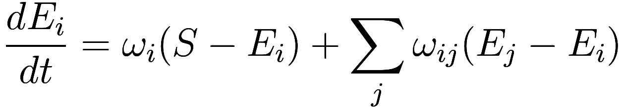
Consider the many physical objects that comprise the surface Earth, such as the vegetation and different layers of the ground and air. Each such component has its own physical characteristics, such as its temperature $E_i$ (which may vary with time), and can be subdivided into further components as necessary. We can linearly approximate the response of $E_i$ to solar forcing, like before, as

$\frac {dE_i}{dt} = \omega_i (S - E_i)$

where $\omega_i$ is the component’s response frequency, which may vary from one component to another. Of course, each of the components interacts in some way with every other, so we have a much bigger system of equations

$\frac {dE_i}{dt} = \omega_i (S - E_i) + \sum_j \omega_{ij} (E_j - E_i)$

We will suppose the $\omega_{ij}$ are generally unimportant compared to the $\omega_i$ : for, if two components interact highly with each other, they are probably in close physical proximity (such as adjacent layers in the ground), so they will respond to solar forcing in a similar way, so they will generally have a similar tempeature anyhow, and heat flow between them is not so important.¹⁰Side note: because $\omega_{ij}$ depends on $1 / C_i$ , where $C_i$ is the heat capacity of the $i$ th component, in general $\omega_{ij} \neq \omega_{ji}$ .

Now, what happens if a solar forcing $S$ with frequency $\omega$ is applied to the system? Each component acts as a low-pass filter with frequency cut-off $\omega_i$ , so $E_i$ will oscillate with $S$ when $\omega_i \gg \omega$ and will not respond when $\omega_i \ll \omega$ . The phase offset of the response is small when $\omega_i \gg \omega$ and approaches a quarter phase when $\omega_i \ll \omega$ .

If you then measure the temperature of the system at some point in time, you will effectively be measuring some sort of an average of the temperatures of its components; this depends on where you are measuring the temperature, and the details of the interaction terms $\omega_{ij}$ that cause changes in the temperature of each component to influence the temperatures of every other one.

Therefore, as sunlight varies over a day, we observe that the parts of the Earth with a very large $\omega_i$ respond to the sunlight by rapidly changing temperature: for example, the top few centimeters of the ground and the bottom few meters of air, which are most directly influenced by sunlight and have a quite low heat capacity. These parts also respond to seasonal variations in sunlight by rapidly changing temperature. If they were the only relevant parts of the surface Earth, then explanation (1) at the very beginning would be correct, and we would observe the hottest part of the year lagging only a few hours behind the brightest part of the year.

However, there are other relevant parts of the Earth, such as the top few meters of ground, top 10-ish km of the troposphere, and the air masses elsewhere on Earth but at the same latitude.¹¹Going even further afield, the yet more distant parts of the Earth have a response timescale even greater than a year, and so are not important to either seasonal or diurnal variations. Their temperatures respond to local variations in sunlight not in hours but in weeks or months, which is too slow for them to be relevant to the diurnal temperature cycle, but not too slow for the seasonal cycle.

Since there are many components to the Earth system with many different characteristic response times to variations in forcing, we expect that forcing of any period will create a lagged response: if there were large weekly or monthly variations in sunlight then the response would be dominated by the portions of the atmosphere with a weekly or monthly characteristic time scale and we would observe the hottest part of the week or month to be moderately after the brightest part. This is what we would expect from most sufficiently messy systems: they will exhibit responses to all frequencies in their input.

Let us conclude by returning to the original question: why is the summer warmer than the winter? Because of the large lag of the hottest day in the summer after the sunniest day in the summer, it must be that the seasonal variation in temperature is dominated by objects that respond to variations in solar heating with a timescale comparable to the seasonal lag. Thus, explanation (2) is (more) correct: the summer is hotter due to the accumulation of more and more heat over the season.

Via radiation of infrared light to space due to the blackbody effect; see my series on the greenhouse effect for more details.↩︎
We suppose that the heat capacity is constant over the range of temperatures of interest, so energy and temperature are linearly related.↩︎
Black-body radiation varies with the fourth power of temperature per the Stefan-Boltzmann law, so we need a cubic correction factor, which is modest over the range of temperatures over interest; but we are not trying to be quantitative yet.↩︎
Indeed this linearity is how we knew that the constant term of $E$ is $S_0$ .↩︎
$\tan x \approx x$ for small $x$ so it is not a surprise that $1 / \omega$ is approximately equal to $t_0$ ↩︎
the angle between the subsolar point and the equator↩︎
The diurnal cycle in solar heating is only poorly approximated by a sine wave; the “effective” daily range should be somewhat larger, but not enough so to change any conclusions.↩︎
Note that the differential equation we’ve been using so far can only produce a phase shift of up to a quarter phase. The reason that temperatures underground can be phase shifted by more than that is that they do not directly interact with the surface, but rather interact via soil at an intermediate depth. Each “layer” of soil is slightly phase shifted and slightly damped relative to the layer above it, so these phase shifts can add up arbitrarily high at depth.↩︎
Additive constants are missing because they considered temperature anomalies $T'$ rather than temperatures $T$ . Note that only a coupling between air and space is explicitly given; there is no explicit insolation term, so the equations as given are only capable of relaxing towards equilibrium. In their numerical simulations, though, they were forced with a step function change in insolation, which is not explicitly shown in the equation. Since their forcing function was a step function instead of sinusoidal, their results were transients instead of periodic.↩︎
Side note: because $\omega_{ij}$ depends on $1 / C_i$ , where $C_i$ is the heat capacity of the $i$ th component, in general $\omega_{ij} \neq \omega_{ji}$ .↩︎
Going even further afield, the yet more distant parts of the Earth have a response timescale even greater than a year, and so are not important to either seasonal or diurnal variations.↩︎

Follow RSS/Atom feed for updates.