This Christmas, while many of us may be admiring the 3-dimensional balls hung on Christmas trees, let us spare a moment to consider the properties of rotations and balls in even dimensions, and how their properties are simplified by pairing up dimensions. Along the way we will find a surprising identity involving the volumes of even-dimensional balls!
The first place many students encounter the dichotomy between even and odd dimensions is in statistics class, when studying the normal distribution. Let
![]()
which is the unnormalized normal distribution: we can think of this
as a kind of “fuzzy” one-dimensional ball. To normalize ![]() we need to calculate its “volume”:
we need to calculate its “volume”:
![]()
The “Gaussian integral” ![]() is a famous problem because the antiderivative of
is a famous problem because the antiderivative of
![]() cannot be expressed in elementary form, but
there is a quite clever trick for finding
cannot be expressed in elementary form, but
there is a quite clever trick for finding ![]() without using the antiderivative. The idea is to
work in two dimensions: as the two-dimensional normal distribution is
rotationally symmetric, we can use the symmetry to convert to polar
coordinates and solve the problem immediately. We demonstrate this
below, where we let
without using the antiderivative. The idea is to
work in two dimensions: as the two-dimensional normal distribution is
rotationally symmetric, we can use the symmetry to convert to polar
coordinates and solve the problem immediately. We demonstrate this
below, where we let ![]() and
and ![]() :
:
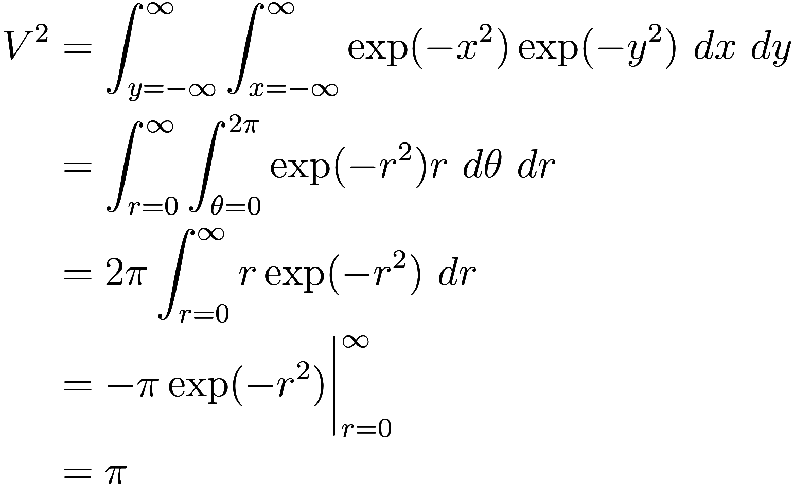
Here the factor of ![]() appears because it is the Jacobian of the
coordinate transformation from Cartesian coordinates to polar
coordinates: a “unit” cell with dimensions
appears because it is the Jacobian of the
coordinate transformation from Cartesian coordinates to polar
coordinates: a “unit” cell with dimensions ![]() by
by ![]() in polar coordinates has an area of
in polar coordinates has an area of ![]() . Formally,
. Formally,
![]()
Thus we find that ![]() or
or ![]() . This
proof is originally due to Poisson, although remarkably it has been
proven that the method shown above (of multiplying a definite integral
by itself) is totally useless for
integrating any other function. This technique is also known in
computer science as the Box-Muller
transform, where it is commonly used to generate random numbers from
a normal distribution: such numbers are generated in pairs, rather than
one at a time.
. This
proof is originally due to Poisson, although remarkably it has been
proven that the method shown above (of multiplying a definite integral
by itself) is totally useless for
integrating any other function. This technique is also known in
computer science as the Box-Muller
transform, where it is commonly used to generate random numbers from
a normal distribution: such numbers are generated in pairs, rather than
one at a time.
We will see this several more times, where the mathematics can be simplified by taking dimensions in pairs instead of singly. The most obvious example of this – complex numbers – will be discussed near the very end.
We have a very strong intuition for rotations in three or fewer dimensions which will not guide us well as we look at higher dimensions.
In one dimension, rotation is not possible: we think of a line as stiff against any possible internal rotation. A creature in one dimension cannot turn around without leaving the line, and is stuck pointing in one direction forever.
In two and three dimensions, a rotation goes around either a point or a line (the “pole”) by a particular angle. If you were to continuously and steadily rotate an object, then after some time (the “rotation period”) it would return to its starting orientation. This is not true above three dimensions!
Fundamentally, the simplest possible rotation takes place in a plane. In three dimensions, you can’t rotate in two different planes at the same time because those planes would intersect in a line, and rotations within a line are impossible. Thus rotations in three dimensions are essentially the same as rotations in two dimensions, except with an extra dimension (the pole) which doesn’t do anything.
In four or more dimensions it is now possible to combine more than
one of these planar rotations at the same time. Thus a single rotation
could involve one plane rotating by ![]() and another plane rotating by
and another plane rotating by ![]() . If you smoothly and steadily rotated a
four-dimensional object, and chose rotation rates that were irrational
multiples of each other, then the object would never return to its
starting orientation.
. If you smoothly and steadily rotated a
four-dimensional object, and chose rotation rates that were irrational
multiples of each other, then the object would never return to its
starting orientation.
Again, rotations in five dimensions are much like rotations in four dimensions with an extra dimension which is fixed.
In general, in ![]() dimensions, for any given rotation
dimensions, for any given rotation ![]() there exists an orthonormal basis
there exists an orthonormal basis ![]() such that
such that ![]() where
where ![]() rotates the plane
rotates the plane ![]() by the angle
by the angle
![]() . That is, any rotation in
. That is, any rotation in ![]() dimensions is a composition of
dimensions is a composition of ![]() rotations, each of which acts on only two
dimensions while leaving the others fixed. These rotations
rotations, each of which acts on only two
dimensions while leaving the others fixed. These rotations ![]() all commute with each other.
all commute with each other.
(In fact, letting the ![]() vary, the group generated by the
vary, the group generated by the ![]() is isomorphic to
is isomorphic to ![]() , and is a maximal torus of
the special
orthogonal group
, and is a maximal torus of
the special
orthogonal group ![]() of all rotations in
of all rotations in ![]() dimensions. In particular, it is a maximal
commutative subgroup of
dimensions. In particular, it is a maximal
commutative subgroup of ![]() : there is no set of
: there is no set of ![]() independent rotations in
independent rotations in ![]() which commute.)
which commute.)
Another way to express this same concept is that in ![]() dimensions, any rotation matrix is similar to a
block diagonal matrix where the blocks are 2 by 2 matrices of the
form:
dimensions, any rotation matrix is similar to a
block diagonal matrix where the blocks are 2 by 2 matrices of the
form:
![]()
This can be proven by noting that the eigenvalues of a rotation all have magnitude 1 (since they are volume-preserving) and come in complex conjugate pairs; so we can diagonalize the matrix in complex numbers and then make pairs of conjugate complex numbers into 2 by 2 blocks of real numbers of the above form.
What happens in ![]() dimensions? Well, it is exactly the same,
except the orthonormal basis has an extra basis element
dimensions? Well, it is exactly the same,
except the orthonormal basis has an extra basis element ![]() which is fixed by
which is fixed by ![]() .
.
A remarkable application of the mathematical theory of rotations arises in the field of crystallography, which curiously stradles the boundary of physics and math. A crystal is a solid object made of a small number of different types of building blocks which are arranged with no “disorder”; that is, their arrangement repeats in a regular way.
(“Disorder” refers to the entropy of the system, and the third law of thermodynamics is often stated that the entropy of a perfect crystal goes to zero as temperature goes to absolute zero. The most common form of ice found on Earth, called icosahedral ice or ice Ih, is actually not a perfect crystal because of the disordered nature of the hydrogen bonds which gives it nonzero entropy at absolute zero. As icosahedral ice is cooled, it can form ice XI, in which the hydrogen bonds are regular.)
The repetitive structure of a crystal is a lattice. Real-world crystal lattices often have some symmetry: for example, table salt has cubic symmetry, which is why chunks of salt tend to come in rectangular shapes. Ice has hexagonal symmetry, causing the six-sided shape of snow flake crystals. However, until 2007, no natural crystal had ever been found with a rotational symmetry other than 2, 3, 4, or 6.
This is a consequence of the crystallographic restriction
theorem, which describes precisely in which dimensions it is
possible to find a lattice with a specified rotational symmetry. Suppose
we want to know in what dimensions there is ![]() -fold rotational symmetry. We factor
-fold rotational symmetry. We factor ![]() into distinct primes as
into distinct primes as
![]()
with ![]() (except possibly for
(except possibly for ![]() ); then the minimum dimension
); then the minimum dimension ![]() with
with ![]() -fold rotational symmetry is
-fold rotational symmetry is
![]()
where the first term is ![]() if
if ![]() and 0 otherwise (this is Iverson bracket
notation). Thus,
and 0 otherwise (this is Iverson bracket
notation). Thus, ![]() is defined identically to the Euler totient
function
is defined identically to the Euler totient
function ![]() except with a sum instead of a product, and
a special case for when
except with a sum instead of a product, and
a special case for when ![]() is twice an odd number.
is twice an odd number.
(Why a sum instead of product? If you have two rotations with coprime
orders that can be performed in ![]() and
and ![]() dimensions, then in
dimensions, then in ![]() dimensions you can perform the first
rotation in the first
dimensions you can perform the first
rotation in the first ![]() dimensions and similarly the second rotation in
the other
dimensions and similarly the second rotation in
the other ![]() dimensions, resulting in a rotation whose order
is the product of their orders.)
dimensions, resulting in a rotation whose order
is the product of their orders.)
For example, ![]() show that five-fold rotations
and eight-fold rotations first arise in four dimensions, and
show that five-fold rotations
and eight-fold rotations first arise in four dimensions, and ![]() shows that seven-fold rotations first
arise in six dimensions.
shows that seven-fold rotations first
arise in six dimensions.
In fact, one sees that each of the terms ![]() and
and ![]() are even, so their sum
are even, so their sum
![]() is always even. Therefore, lattice
symmetries of order
is always even. Therefore, lattice
symmetries of order ![]() first arise in an even dimension, and an
odd-dimensional space doesn’t have any new lattice symmetries that were
absent from the previous dimension.
first arise in an even dimension, and an
odd-dimensional space doesn’t have any new lattice symmetries that were
absent from the previous dimension.
A nascent development in crystallography is the discovery of quasicrystals, which are crystals that violate the crystallographic restriction theorem. These quasicrystals are described by quasilattices, which are not mathematical lattices, but share some of the same properties. Quasilattices are formed by taking an imperfect slice of a higher-dimensional lattice: in this way they acquire forbidden symmetries by taking them from a higher dimension, but the slicing process gives them a sort of regular pattern of imperfections that make them not a true lattice. The most popular example of such a quasilattice is the Penrose tiling:
The Penrose tiling. It has five-fold symmetry, which is forbidden in two dimensions for regular lattices. Image from wikipedia.
The first quasicrystal to be made in the lab was in 1982. The first naturally discovered quasicrystal was in a meteorite in 2007. The only commercial application of quasicrystals so far has been as a non-stick frying pan coating.
A Ho-Mg-Zn quasicrystal. Image from wikipedia.
Recall the definition of the unit ![]() -ball,
-ball,
![]()
and let ![]() be its volume. Certainly the
be its volume. Certainly the ![]() -ball with radius
-ball with radius ![]() has volume
has volume ![]() .
.
We can find ![]() as an integral iterated
as an integral iterated ![]() times, integrating once over each coordinate,
which can be readily solved using induction. Surprisingly (or not?), the
induction is easiest when inducting by two dimensions at a time.
times, integrating once over each coordinate,
which can be readily solved using induction. Surprisingly (or not?), the
induction is easiest when inducting by two dimensions at a time.
Given ![]() , we aim to calculate
, we aim to calculate ![]() . Let
. Let ![]() be the two new
coordinates, and let
be the two new
coordinates, and let ![]() and
and ![]() so that
so that ![]() consists of the points where
consists of the points where ![]() . Then we have
. Then we have
![\begin{aligned}
V(n + 2) &= \int_{r^2 < 1} \left[ \int_{x_1^2 + \cdots + x_n^2 < s^2}\ dx_1 \cdots dx_n \right]\ du\ dv \\
&= \int_{r^2 < 1} V(n) s^n \ du\ dv \\
&= V(n) \int_{r = 0}^1 \int_{\thet...](../a/1e099984e907543d.png)
where we converted from Cartesian ![]() coordinates to polar coordinates by
coordinates to polar coordinates by ![]() as before. Now if
as before. Now if ![]() , we have
, we have ![]() , so
, so
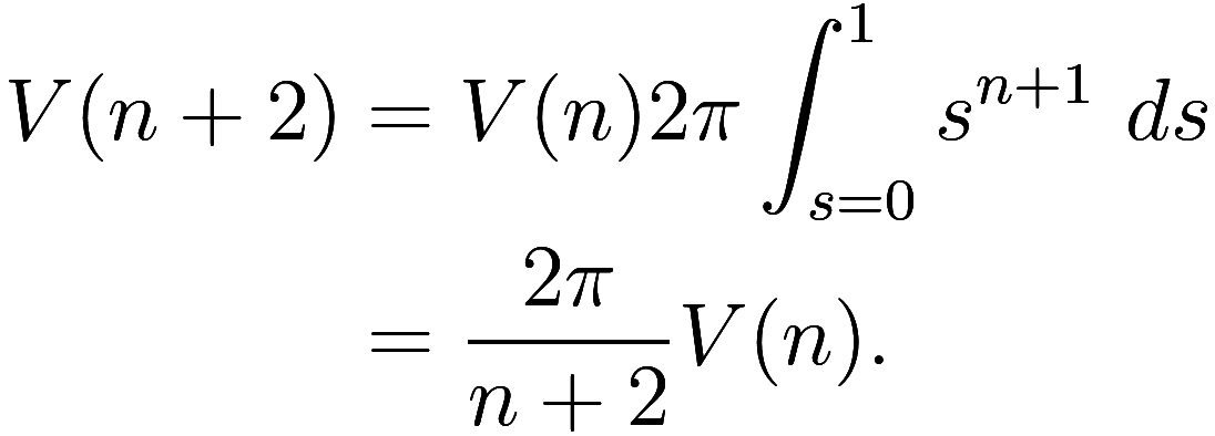
Since ![]() , it follows that
, it follows that
![]()
Thus the volume of the ![]() -ball decreases faster than exponentially for large
-ball decreases faster than exponentially for large
![]() , and so the sum of the volumes of the
even-dimensional balls must converge. We find that
, and so the sum of the volumes of the
even-dimensional balls must converge. We find that
![]()
and in fact if we use balls with radius ![]() instead of unit balls, the sum of those volumes is
instead of unit balls, the sum of those volumes is
![]() . As a special case, when we use the
radius
. As a special case, when we use the
radius ![]() , the sum of the volumes is
, the sum of the volumes is ![]() !
!
For completeness sake, we can use ![]() to find
to find
![]()
The common cause for each of these phenomena is the repeated use of 2 in the exponents in several equations, such as the formula for the normal distribution and the Pythagorean formula for finding the distance a point is from the origin.
This becomes apparent by generalizing our definition of distance. In
the ![]() -norm, the distance
-norm, the distance ![]() of a point
of a point ![]() from the origin is
from the origin is
![]()
with ![]() giving us the ordinary
giving us the ordinary ![]() -norm. This is defined for
-norm. This is defined for ![]() ; in the case
; in the case ![]() we say that
we say that ![]() .
.
When ![]() is an integer, we can evaluate the
“Gaussian”-like integral
is an integer, we can evaluate the
“Gaussian”-like integral ![]() by taking the integral to the power of
by taking the integral to the power of
![]() (the particular case
(the particular case ![]() can be evaluated directly with no special
tricks), and the volume of the ball can be inductively calculated by
inducting by
can be evaluated directly with no special
tricks), and the volume of the ball can be inductively calculated by
inducting by ![]() dimensions at a time.
dimensions at a time.
We explicitly show how to do the latter calculation. Let
![]()
the definition of the ![]() -ball in the
-ball in the ![]() -norm. Let
-norm. Let ![]() be its volume. As before, we calculate
be its volume. As before, we calculate ![]() from
from ![]() : let
: let ![]() be the
coordinates in
be the
coordinates in ![]() dimensions, with
dimensions, with
![]()
and ![]() . Then, as before
. Then, as before
![]()
Now the coordinate change is a little messier, because we are no
longer using polar coordinates but rather converting to coordinates for
the ![]() -ball in the
-ball in the ![]() -norm. Let
-norm. Let ![]() be the surface area of the
be the surface area of the ![]() -ball in the
-ball in the ![]() -norm, so that
-norm, so that
![]()
Then we have
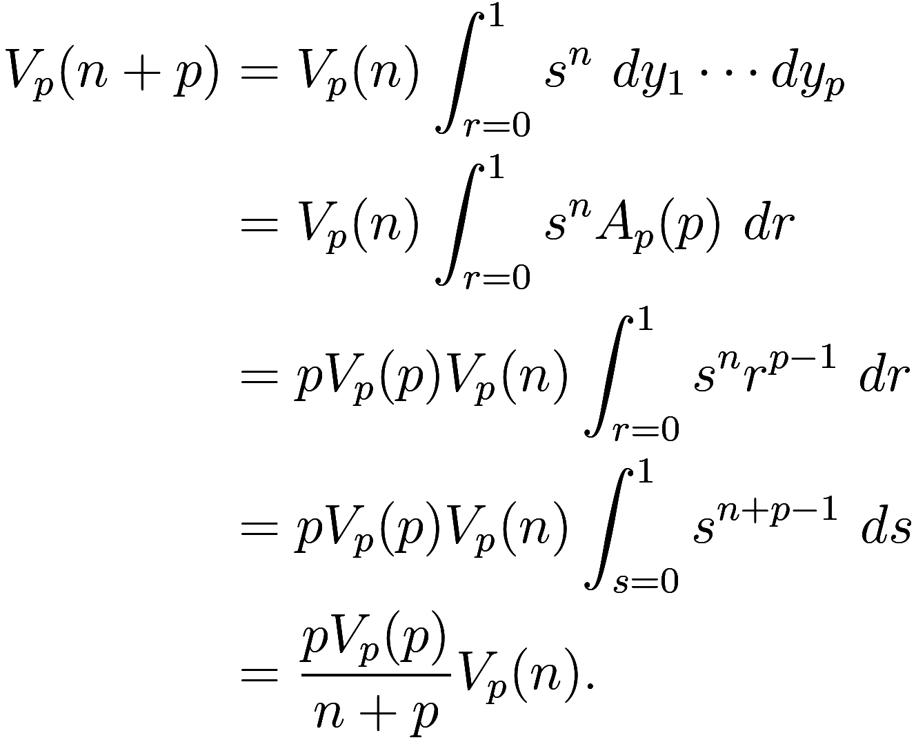
Thus in the same way we have a recurrence from ![]() to
to ![]() when using the
when using the ![]() -norm. To actually use this, we need the
value of
-norm. To actually use this, we need the
value of ![]() . I was unable to easily make progress
computing this, but found a paper (Volumes of generalized unit
balls) with the result:
. I was unable to easily make progress
computing this, but found a paper (Volumes of generalized unit
balls) with the result:
![]()
(The paper calculates ![]() by inducting over
by inducting over ![]() one at a time. The resulting integrals are rather
messy compared to the above, but with suitable changes of variable can
be made into gamma functions.)
one at a time. The resulting integrals are rather
messy compared to the above, but with suitable changes of variable can
be made into gamma functions.)
Combining with the inductive relationship, we get
![]()
As lattice symmetries, and thus the crystallographic restriction
theorem, are consequences of the properties of rotations in ![]() dimensions, this leaves us only with the question
of why pairs of numbers are important to rotations.
dimensions, this leaves us only with the question
of why pairs of numbers are important to rotations.
Rotations are isometries: they preserve distance. (They are
also orientation-preserving, that is, don’t make mirror images, but that
is not important here). “Distance” here means, as one expects, the
ordinary distance in the ![]() -norm.
-norm.
Since rotations are defined with respect to the ![]() -norm, it is natural that the pairing up of
dimensions is important to rotations. However, unlike the case with
volumes of
-norm, it is natural that the pairing up of
dimensions is important to rotations. However, unlike the case with
volumes of ![]() -balls, there does not seem to be any sensible way
to define rotations with respect to the
-balls, there does not seem to be any sensible way
to define rotations with respect to the ![]() -norm for
-norm for ![]() . Such
a space only has trivial isometries (those that permute or negate
the coordinates), and it seems that any non-trivial way of creating
isometries in
. Such
a space only has trivial isometries (those that permute or negate
the coordinates), and it seems that any non-trivial way of creating
isometries in ![]() essentially amounts to partially using
an
essentially amounts to partially using
an ![]() -norm and getting some subset of the usual
isometries.
-norm and getting some subset of the usual
isometries.
Now what makes the ![]() -norm so special that it is the only way to
usefully define rotations? This brings us to the glaring omission in our
discussion so far: the complex numbers. Complex numbers are the clearest
example in mathematics of when taking a pair of real numbers can greatly
simplify a situation that is challenging for single real numbers. While
the link between complex numbers and isometries is not readily apparent,
as what makes complex numbers unique is their algebraic
properties rather than their metric properties, I hope to
elucidate what I believe is the key connection.
-norm so special that it is the only way to
usefully define rotations? This brings us to the glaring omission in our
discussion so far: the complex numbers. Complex numbers are the clearest
example in mathematics of when taking a pair of real numbers can greatly
simplify a situation that is challenging for single real numbers. While
the link between complex numbers and isometries is not readily apparent,
as what makes complex numbers unique is their algebraic
properties rather than their metric properties, I hope to
elucidate what I believe is the key connection.
Consider a linear transformation ![]() . For
. For ![]() to be an isometry it needs to preserve the length
of any element of
to be an isometry it needs to preserve the length
of any element of ![]() , including in particular its
eigenvectors. Thus, its eigenvalues must all have magnitude 1. The
eigenvalues of
, including in particular its
eigenvectors. Thus, its eigenvalues must all have magnitude 1. The
eigenvalues of ![]() can be found from its characteristic
polynomial:
can be found from its characteristic
polynomial:
![]()
The roots of ![]() are the eigenvalues of
are the eigenvalues of ![]() . Finding the roots of a polynomial is an
essentially algebraic operation, and for
. Finding the roots of a polynomial is an
essentially algebraic operation, and for ![]() to always have
to always have ![]() roots requires moving from
roots requires moving from ![]() to its algebraic closure
to its algebraic closure ![]() : working in the real numbers, the most we
can guarantee that
: working in the real numbers, the most we
can guarantee that ![]() can be factored is into terms that are
quadratic or less. These quadratic terms correspond exactly to the
planes within which
can be factored is into terms that are
quadratic or less. These quadratic terms correspond exactly to the
planes within which ![]() rotates.
rotates.
Each eigenvalue ![]() must have magnitude 1 for
must have magnitude 1 for
![]() to be an isometry. Which norm should we use to
calculate the magnitude of
to be an isometry. Which norm should we use to
calculate the magnitude of ![]() ? For the finite extension
? For the finite extension ![]() there is only one natural
choice of norm, given by taking the product of all of the conjugates of
there is only one natural
choice of norm, given by taking the product of all of the conjugates of
![]() . If
. If ![]() , we have
, we have
![]()
In this way, we see that the ![]() -norm is inextricably linked to the complex
numbers and to isometries in
-norm is inextricably linked to the complex
numbers and to isometries in ![]() .
.
Even if we try to move from the real numbers to another number
system, we run into the Artin-Schreier
Theorem: if ![]() is a proper subfield of the complex numbers with
finite index, then the index is 2 and
is a proper subfield of the complex numbers with
finite index, then the index is 2 and ![]() , so exactly the same norm
, so exactly the same norm
![]() would be used. Furthermore, any finite
extension of a field in its algebraic closure has this same property and
is essentially like the real numbers in the complex numbers. Finally,
since
would be used. Furthermore, any finite
extension of a field in its algebraic closure has this same property and
is essentially like the real numbers in the complex numbers. Finally,
since ![]() is algebraically closed, it has no finite
extensions, so we can’t build larger finite extensions of the real
numbers.
is algebraically closed, it has no finite
extensions, so we can’t build larger finite extensions of the real
numbers.
Thus in a fundamental sense all finite dimensional rotations involve
repeated copies of the Argand plane
representation of the complex numbers, where multiplying by ![]() rotates by an angle of
rotates by an angle of ![]() .
.
Another remarkable example of simplifying rotations by moving from an odd number of dimensions to an even number is the application of quaternions to simplify the computation of rotations in three dimensions.
As we saw above, any individual rotation in three dimensions can be described as a pole which remains fixed together with an angle in the plane of rotation. If two different rotations have the same pole, they commute with each other and we can compose them by simply adding angles: this is the simple circumstance of rotations in two dimensions. However the general problem of composing rotations in three dimensions requires some thought.
The space ![]() of rotations has three dimensions, so
we can describe any rotation with three numbers, and there are many ways
to do so. The most obvious ways are the axis-angle
representation described above, Euler angles which
describe a rotation in terms of a succession of rotations around the
three coordinate axes, and Tait-Bryan angles which are another way of
composing rotations around the three coordinate axes.
of rotations has three dimensions, so
we can describe any rotation with three numbers, and there are many ways
to do so. The most obvious ways are the axis-angle
representation described above, Euler angles which
describe a rotation in terms of a succession of rotations around the
three coordinate axes, and Tait-Bryan angles which are another way of
composing rotations around the three coordinate axes.
Besides the difficulty of computing the composition of two rotations
given in the above systems, any chart representing ![]() with three numbers cannot cover the
whole space of rotations without singularities. These singularities
result in gimbal
lock, which is a phenomenon in which the coordinate system becomes
linearly dependent, and certain degrees of freedom cannot be expressed
at the singularities. In addition to being a mathematical problem, this
happens to real-world gyroscopes when only three gimbals are used: the
positions of the three gimbals is a representation of a rotation with
three coordinates, and their exists orientations in which some of the
gimbals become redundant, and the gyroscope locks up against rotation in
a specific direction. This physical limitation meant that (some of) the
Apollo spacecraft would lose orientation information if pointed in
specific directions. In fact, when the damaged Apollo 13 was descending
to Earth its astronauts were forced
to jetison the lunar module (see also: part
1) prematurely because its automatic attitude adjustment was sending
the command module too close to gimbal lock, which would have endangered
the final descent trajectory.
with three numbers cannot cover the
whole space of rotations without singularities. These singularities
result in gimbal
lock, which is a phenomenon in which the coordinate system becomes
linearly dependent, and certain degrees of freedom cannot be expressed
at the singularities. In addition to being a mathematical problem, this
happens to real-world gyroscopes when only three gimbals are used: the
positions of the three gimbals is a representation of a rotation with
three coordinates, and their exists orientations in which some of the
gimbals become redundant, and the gyroscope locks up against rotation in
a specific direction. This physical limitation meant that (some of) the
Apollo spacecraft would lose orientation information if pointed in
specific directions. In fact, when the damaged Apollo 13 was descending
to Earth its astronauts were forced
to jetison the lunar module (see also: part
1) prematurely because its automatic attitude adjustment was sending
the command module too close to gimbal lock, which would have endangered
the final descent trajectory.
A gyroscope with three gimbals. Image from wikipedia.
The clever trick to solve this problem is to use four coordinates
instead of three. The unit sphere in four dimensions is a double-cover
of ![]() , so that we can represent a rotation
as a vector of four numbers
, so that we can represent a rotation
as a vector of four numbers ![]() subject to the condition that
subject to the condition that ![]() ; any particular rotation has exactly
two such representations. The surprising feature of this representation
is that if we view the vector as a quaternion
; any particular rotation has exactly
two such representations. The surprising feature of this representation
is that if we view the vector as a quaternion ![]() , then composition
of two rotations is exactly the same as quaternion
multiplication.
, then composition
of two rotations is exactly the same as quaternion
multiplication.
Quaternions thus give another example of simplifying a problem involving rotations by moving from an odd number of dimensions to an even number. However, any deeper link between the quaternions and the examples given above has eluded me, and for now I can only explain it as a coincidence.
Addendum: reddit user AntiTwister suggested this accessible and informative article which gives the insight to explain why quaternions represent rotations and the appropriate generalization rotors (see geometric algebra) to rotations in any number of dimensions.
Follow RSS/Atom feed for updates.