(As mentioned before, current MIT students should not read this material.)
Having looked at how the largest cluster size ![]() varies with
varies with ![]() for a fixed
for a fixed ![]() , now we consider the converse of what happens as
, now we consider the converse of what happens as
![]() varies for a fixed
varies for a fixed ![]() .
.
We learned in class that ![]() follows certain functional forms in the limit
of large
follows certain functional forms in the limit
of large ![]() :
:
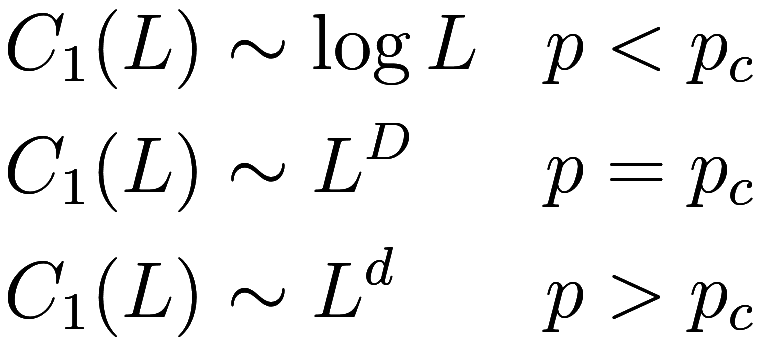
Here, ![]() is the dimension of the grid being used, and
is the dimension of the grid being used, and ![]() is the fractal dimension of the
critical percolating cluster1The
fractal scaling
is the fractal dimension of the
critical percolating cluster1The
fractal scaling ![]() is just one of many power laws that describe
the behavior of a percolating cluster at or near the critical point. The
exponents of these power laws are referred to as “universal”
critical exponents because their value does not depend on the local
shape of the grid being used as a substrate, but only on the grid’s
dimension; thus all two-dimensional grids follow the same power laws.
For
is just one of many power laws that describe
the behavior of a percolating cluster at or near the critical point. The
exponents of these power laws are referred to as “universal”
critical exponents because their value does not depend on the local
shape of the grid being used as a substrate, but only on the grid’s
dimension; thus all two-dimensional grids follow the same power laws.
For ![]() , the exponents stop depending on the
dimension, and equal the values according to mean-field
theory. Generally speaking we only have exact results for
, the exponents stop depending on the
dimension, and equal the values according to mean-field
theory. Generally speaking we only have exact results for ![]() , where conformal
field theory can be used, or
, where conformal
field theory can be used, or ![]() where mean-field theory is
correct..
where mean-field theory is
correct..
As an aside, it is worth noting that this behavior for ![]() is not obvious, and it is plausible for there
to exist a range of values of
is not obvious, and it is plausible for there
to exist a range of values of ![]() which exhibit large clusters2i.e.,
cluster sizes distributed like a power law, and therefore
which exhibit large clusters2i.e.,
cluster sizes distributed like a power law, and therefore ![]() would be a power law in
would be a power law in ![]() without having infinite clusters.
It wasn’t until the 1980s that is was proved3eg “Sharpness
of the Phase Transition in Percolation Models” by Michael Aizenman
and David J. Barsky that there was a single phase
transition at a single critical point
without having infinite clusters.
It wasn’t until the 1980s that is was proved3eg “Sharpness
of the Phase Transition in Percolation Models” by Michael Aizenman
and David J. Barsky that there was a single phase
transition at a single critical point ![]() at which clusters go immediately from being
small to infinite.
at which clusters go immediately from being
small to infinite.
Can we observe these functional forms empirically? Let us start in
2D, and graph how ![]() and
and ![]() (the second-largest cluster size) vary with
(the second-largest cluster size) vary with
![]() for
for ![]() .
.
We have shown the least-squares fit of ![]() as a linear function of
as a linear function of ![]() for large
for large ![]() ; it is quite a good fit.
; it is quite a good fit. ![]() also appears to grow like
also appears to grow like ![]() , although I did not perform a fit.
, although I did not perform a fit.
Moving up to ![]() :
:
We are now fitting ![]() against two different functional forms. Where
against two different functional forms. Where
![]() is almost as large as one would expect at the
critical point, we are fitting
is almost as large as one would expect at the
critical point, we are fitting ![]() against a power law; where
against a power law; where ![]() is significantly smaller than one expects at
the critical point, we fit against
is significantly smaller than one expects at
the critical point, we fit against ![]() 4Specifically, we use a power law where
4Specifically, we use a power law where ![]() is at least 80% of
is at least 80% of ![]() at
at ![]() for that
for that ![]() , and
, and ![]() where
where ![]() is at most 20% of
is at most 20% of ![]() at
at ![]() for that
for that ![]() .. Again, for large
.. Again, for large ![]() we see that
we see that ![]() is a good fit against
is a good fit against ![]() .
.
At ![]() :
:
It is hard to say at this point that ![]() is a good fit for
is a good fit for ![]() ; at this point it is looking more and more
like a power law.
; at this point it is looking more and more
like a power law.
Finally we get to ![]() :
:
An excellent fit to a power law! Or at least, it looks like
an excellent fit until it is compared to the fit with ![]() , very close to
, very close to ![]() :
:
I find it remarkable how much of a difference there is between 0.59
and 0.5927; the former has a very slight but visible bend to the graph
as ![]() starts to fall behind slightly for large
starts to fall behind slightly for large ![]() . Also, one can see that
. Also, one can see that ![]() and
and ![]() are not quite parallel when
are not quite parallel when ![]() ;
; ![]() is slowly but surely catching up on
is slowly but surely catching up on ![]() . But at
. But at ![]() however,
however, ![]() and
and ![]() both perfectly match a power law for as high a
value of
both perfectly match a power law for as high a
value of ![]() as my computer could handle, and visually appear
exactly parallel5Though
from the exponent we see
as my computer could handle, and visually appear
exactly parallel5Though
from the exponent we see ![]() is in fact slightly catching up on
is in fact slightly catching up on ![]() . This is because at
. This is because at ![]() the system exhibits scale
invariance.
the system exhibits scale
invariance.
What of the fractal dimension? We estimate ![]() , just shy of the correct value known to be exactly
, just shy of the correct value known to be exactly
![]() .
.
Continuing, as soon as ![]() it is already obvious we have overshot
it is already obvious we have overshot
![]() :
:
And it just gets more obvious as ![]() increases; at
increases; at ![]() the second-largest cluster can no longer
keep up:
the second-largest cluster can no longer
keep up:
Here we see that ![]() , very close to the predicted
relation of
, very close to the predicted
relation of ![]() for
for ![]() .
.
Of course, the same observations hold in 3D. Here is the behavior at the critical point:
Now we can use these graphs to resolve a bit of a mystery. We saw
previously that for any fixed ![]() ,
, ![]() varies continuously as a function of
varies continuously as a function of ![]() . However, the theoretical functional forms for
. However, the theoretical functional forms for
![]() do not vary continuously: they abruptly change
from
do not vary continuously: they abruptly change
from ![]() when
when ![]() to a power law at
to a power law at ![]() . How can we resolve this disparity?
. How can we resolve this disparity?
It appears from these graphs that we were wrong about the
functional forms, and the functional form actually does change
continuously; first ![]() fits
fits ![]() well for small
well for small ![]() , then gradually becomes more like a power law as
, then gradually becomes more like a power law as
![]() approaches
approaches ![]() . However this isn’t true – the functional forms
as stated above are correct. What actually happens is that although the
functional form for large
. However this isn’t true – the functional forms
as stated above are correct. What actually happens is that although the
functional form for large ![]() does abruptly change at
does abruptly change at ![]() , as
, as ![]() gets closer to
gets closer to ![]() then how large
then how large ![]() needs to be for the functional form to be
applicable grows considerably.
needs to be for the functional form to be
applicable grows considerably.
This is related to the notion of uniform
convergence; while ![]() is a continuous function of
is a continuous function of ![]() for any fixed
for any fixed ![]() , as we take the limit
, as we take the limit ![]() ,
, ![]() converges to a discontinuous function. This is
because the convergence is not uniform,6necessarily, as uniform convergence of
continuous functions always gives a continuous function
but rather the convergence is slower for
converges to a discontinuous function. This is
because the convergence is not uniform,6necessarily, as uniform convergence of
continuous functions always gives a continuous function
but rather the convergence is slower for ![]() near
near ![]() .
.
How large ![]() needs to be to be considered “large” is called
the correlation
length
needs to be to be considered “large” is called
the correlation
length ![]() ; we find it by asking the question, what is the
probability that two occupied sites belong to the same cluster7More
rigorously, how much more likely are they to be in the same
cluster than two far-away points are in the same cluster? This is the
same question when
; we find it by asking the question, what is the
probability that two occupied sites belong to the same cluster7More
rigorously, how much more likely are they to be in the same
cluster than two far-away points are in the same cluster? This is the
same question when ![]() , but for
, but for ![]() two distant points have a nonzero chance
of lying in the same cluster because there is an infinite cluster. Thus
what we are really asking is the chance two sites lie in the same
finite cluster.? If they are further than
two distant points have a nonzero chance
of lying in the same cluster because there is an infinite cluster. Thus
what we are really asking is the chance two sites lie in the same
finite cluster.? If they are further than ![]() apart, the probability falls exponentially with
the distance between them, like
apart, the probability falls exponentially with
the distance between them, like ![]() . Another way to see this is that the
radius of a random cluster tends to be at most around
. Another way to see this is that the
radius of a random cluster tends to be at most around ![]() 8or a
suitable power thereof.
8or a
suitable power thereof.
Therefore when ![]() is as big as
is as big as ![]() , the largest finite clusters tend to
span the whole grid, and the system behaves roughly as if it were at
, the largest finite clusters tend to
span the whole grid, and the system behaves roughly as if it were at
![]() . Only for
. Only for ![]() can we observe the limiting behavior.
can we observe the limiting behavior.
![]() itself obeys a power-law relationship (see the
above footnote on universal critical percolation exponents):
itself obeys a power-law relationship (see the
above footnote on universal critical percolation exponents):
![]()
where ![]() for all 2D grids. Thus when
for all 2D grids. Thus when ![]() we find
we find ![]() and would need
and would need ![]() to be significantly larger than that to observe
the
to be significantly larger than that to observe
the ![]() behavior, whereas our graph only extended to
behavior, whereas our graph only extended to
![]() .
.
We can see this with a 3D plot of ![]() :
:
The ramp region with ![]() corresponds to a power law growth rate,
and the constant slope of 2 shows that that whole region has the same
exponent of
corresponds to a power law growth rate,
and the constant slope of 2 shows that that whole region has the same
exponent of ![]() . The flatter region with
. The flatter region with ![]() has an asymptotic growth rate of
has an asymptotic growth rate of ![]() . As
. As ![]() gets larger, the transition between the flat
region and the ramp becomes sharper and sharper, but for any fixed value
of
gets larger, the transition between the flat
region and the ramp becomes sharper and sharper, but for any fixed value
of ![]() it remains continuous and unbroken.
it remains continuous and unbroken.
The ![]() behavior for
behavior for ![]() is clear, as each occupied site has some
fixed, high probability
is clear, as each occupied site has some
fixed, high probability ![]() of being in the big cluster, so
of being in the big cluster, so ![]() scales with the volume of the domain
scales with the volume of the domain
![]() . To understand the transition from
. To understand the transition from ![]() to
to ![]() better let us see if we can explain the
better let us see if we can explain the ![]() behavior.
behavior.
The key observation is that when ![]() , far away sites are unlikely to belong
to the same cluster; the probability decays exponentially with distance
between the sites, so as
, far away sites are unlikely to belong
to the same cluster; the probability decays exponentially with distance
between the sites, so as ![]() most sites become uncorrelated. Thus
we can imagine each of the clusters as being (mostly) independent of
each other. There is some finite average size for a cluster, so as
most sites become uncorrelated. Thus
we can imagine each of the clusters as being (mostly) independent of
each other. There is some finite average size for a cluster, so as ![]() is increased the number of clusters
is increased the number of clusters ![]() grows proportionally to the volume of the
domain:
grows proportionally to the volume of the
domain:
![]()
So to find the largest cluster, imagine taking ![]() iid samples
iid samples ![]() from some probability distribution
from some probability distribution
![]() of cluster sizes.
of cluster sizes. ![]() will be somewhat “nice” in that it has finite
mean, finite variance, and goes to 0 rapidly as
will be somewhat “nice” in that it has finite
mean, finite variance, and goes to 0 rapidly as ![]() .
.
Let ![]() be the maximum of the
be the maximum of the ![]() ; we wish to find the probability distribution
; we wish to find the probability distribution
![]() of
of ![]() . Now certainly by definition of
. Now certainly by definition of ![]() ,
,
![]()
where we have used independence of the ![]() and identity of the
and identity of the ![]() . Note that
. Note that ![]() is simply the cumulative distribution
function of
is simply the cumulative distribution
function of ![]() , i.e., its integral.
, i.e., its integral.
Let ![]() be the median of
be the median of ![]() . Then
. Then
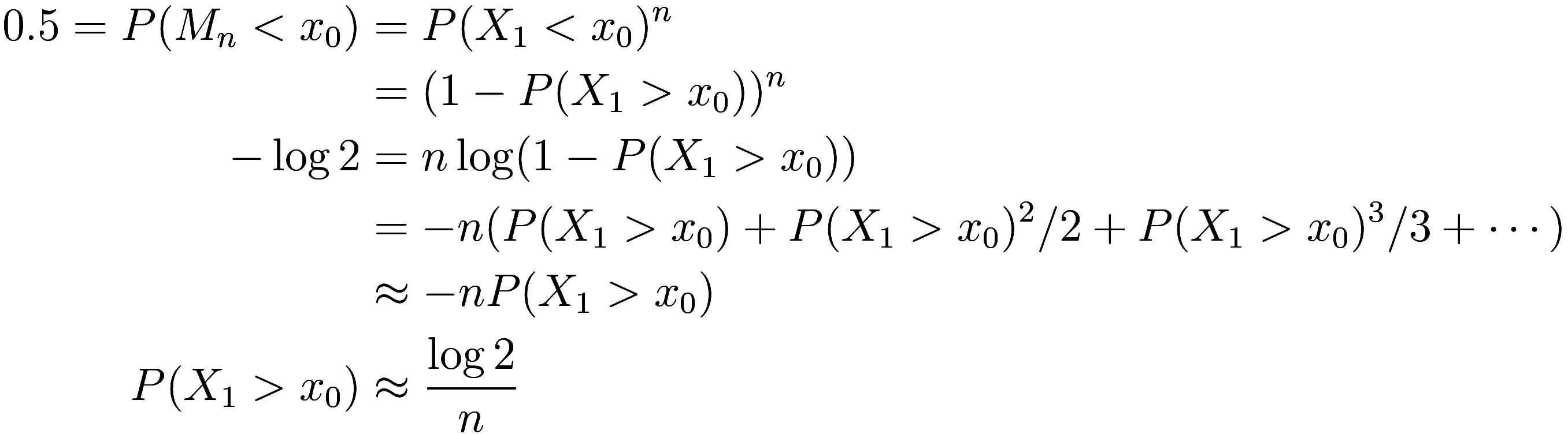
We have used the Taylor series for ![]() ; the approximation is accurate because
; the approximation is accurate because ![]() is extremely large and so
is extremely large and so ![]() is extremely small.
is extremely small.
So now we need to know the asymptotic behavior of ![]() . A logical guess is that
. A logical guess is that ![]() is a normal distribution. In that case, its cdf
is called the error function
(after scaling and translating appropriately), in this context more
specifically called the Q-function. An
excellent approximation for the tail behavior of
is a normal distribution. In that case, its cdf
is called the error function
(after scaling and translating appropriately), in this context more
specifically called the Q-function. An
excellent approximation for the tail behavior of ![]() is
is ![]() where
where ![]() is the standard normal distribution, so we
get
is the standard normal distribution, so we
get
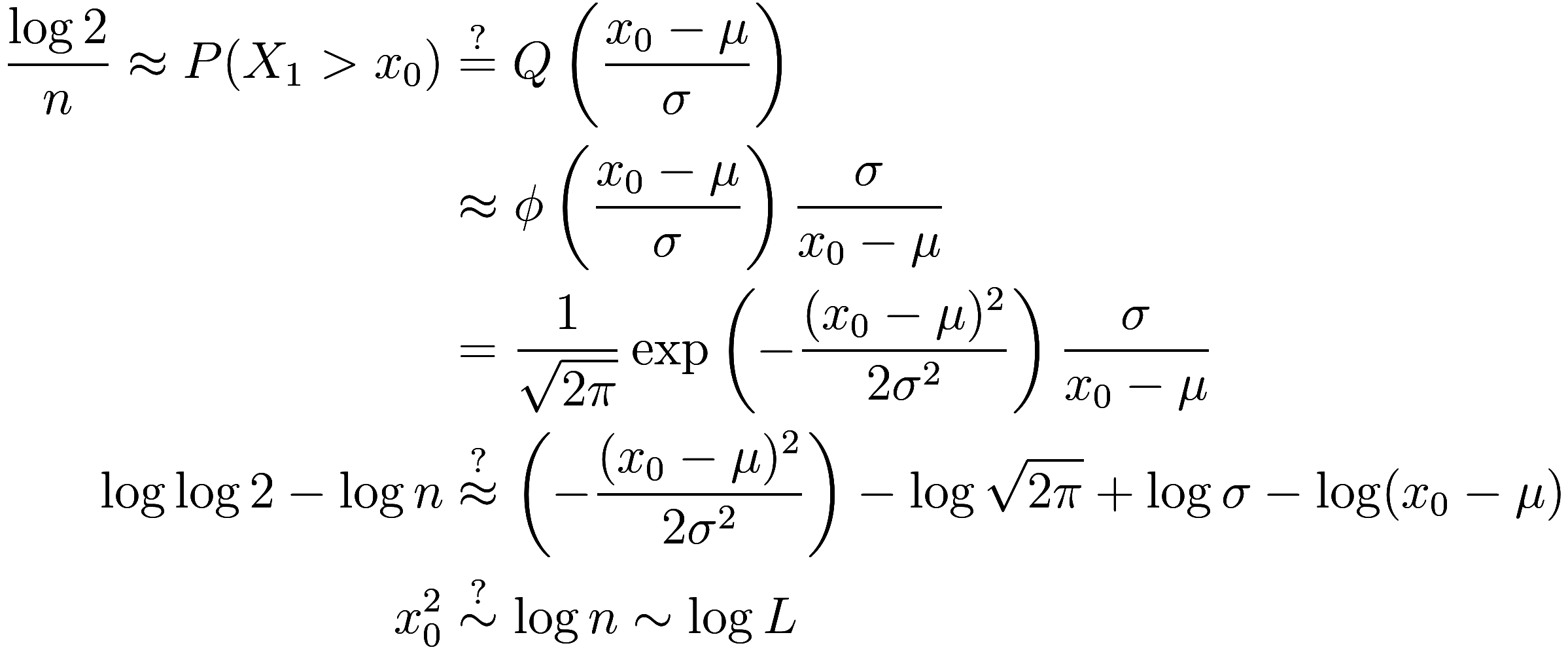
Recall ![]() is the median of the maximum cluster size, and
that
is the median of the maximum cluster size, and
that ![]() . In the end we find that
. In the end we find that ![]() … which is not correct!
… which is not correct!
So our guess that cluster sizes are normally distributed is not good; the normal distribution has too little weight in the tails.
Let us see if we can derive the tail behavior of ![]() from first principles. To start, suppose we are
in 1D, and we have
from first principles. To start, suppose we are
in 1D, and we have ![]() .
.
Consider an occupied site, and for simplicity ignore its left
neighbor. For it to be part of a cluster of size ![]() , the
, the ![]() sites to the right must all be occupied,
which has probability
sites to the right must all be occupied,
which has probability ![]() . Each step further imposes another factor
of
. Each step further imposes another factor
of ![]() , so
, so ![]() is an exponential distribution. That is,
is an exponential distribution. That is, ![]() , and likewise its integral
, and likewise its integral ![]() . This gives:
. This gives:
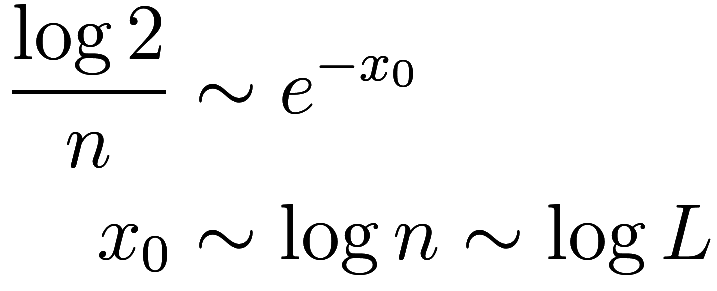
which is now correct.
What about higher than 1D? The whole difficulty with ![]() is the presence of loops in the grid,
i.e., there is more than one route between any two particular sites. If
there were only one route connecting two sites it would be very easy to
predict whether they are in the same cluster.
is the presence of loops in the grid,
i.e., there is more than one route between any two particular sites. If
there were only one route connecting two sites it would be very easy to
predict whether they are in the same cluster.
Thus we turn to the Bethe lattice,
which is the infinite tree where each vertex has ![]() neighbors. If we take
neighbors. If we take ![]() , then the Bethe lattice strongly resembles
the
, then the Bethe lattice strongly resembles
the ![]() -dimensional grid, in that both are regular graphs
with vertex degree
-dimensional grid, in that both are regular graphs
with vertex degree ![]() . In fact, the Bethe lattice is the universal
covering graph of the integer lattice; that is, it was what you get
when removing all the loops from the integer lattice. E.g., if you go
up, right, down, left on the Bethe lattice you do not return where you
started – the only way to return to the origin is to exactly retrace
your steps.
. In fact, the Bethe lattice is the universal
covering graph of the integer lattice; that is, it was what you get
when removing all the loops from the integer lattice. E.g., if you go
up, right, down, left on the Bethe lattice you do not return where you
started – the only way to return to the origin is to exactly retrace
your steps.
The Bethe lattice being a tree, there is a unique path connecting any
two sites, which again makes it easy to calculate the cluster size
distribution. An occupied site has ![]() neighbors, each with a probability
neighbors, each with a probability ![]() of being occupied. Each “newly” occupied neighbor
opens up an additional
of being occupied. Each “newly” occupied neighbor
opens up an additional ![]() new neighbors which have the potential to be
occupied themselves. We can model this process of growing a cluster as a
weighted random walk that starts
new neighbors which have the potential to be
occupied themselves. We can model this process of growing a cluster as a
weighted random walk that starts ![]() units to the right of the origin and at each time
step has a
units to the right of the origin and at each time
step has a ![]() probability of going
probability of going ![]() units to the right and
units to the right and ![]() probability going 1 unit to the left; the
size of the cluster is one plus the number of times the random walk went
to the right before reaching the origin.9The
distance from the origin represents the number of sites adjacent to the
incomplete cluster that have not yet been determined whether they are
occupied or not. Thus the size of the cluster is
probability going 1 unit to the left; the
size of the cluster is one plus the number of times the random walk went
to the right before reaching the origin.9The
distance from the origin represents the number of sites adjacent to the
incomplete cluster that have not yet been determined whether they are
occupied or not. Thus the size of the cluster is ![]() where
where ![]() is the time it takes for the random walk to reach
the origin.
is the time it takes for the random walk to reach
the origin.
For ![]() , which is the critical threshold
for the Bethe lattice, this random walk is biased towards the left. The
path of a biased random walk can be thought of as diffusing from a mean
position which is moving with time. For large times
, which is the critical threshold
for the Bethe lattice, this random walk is biased towards the left. The
path of a biased random walk can be thought of as diffusing from a mean
position which is moving with time. For large times ![]() , this mean position is
, this mean position is ![]() to the left of the origin (specifically, the
mean position is at
to the left of the origin (specifically, the
mean position is at ![]() ), but the standard deviation
only grows like
), but the standard deviation
only grows like ![]() , like all random walks / diffusion
processes. Therefore to remain to the right of the origin at time
, like all random walks / diffusion
processes. Therefore to remain to the right of the origin at time ![]() requires being
requires being ![]() standard deviations to the right. Since
diffusion
creates a normal distribution, the probability of remaining
standard deviations to the right. Since
diffusion
creates a normal distribution, the probability of remaining ![]() standard deviations from the mean scales
like
standard deviations from the mean scales
like
![]()
which is an exponential decay, exactly as we saw in 1D (recall that the time it takes this random walk to cross the origin is proportional to the size of the cluster).
Thus we have recovered the desired ![]() scaling for clusters in the Bethe lattice,
but how does this help us with the standard integer lattice when
scaling for clusters in the Bethe lattice,
but how does this help us with the standard integer lattice when ![]() ?
?
Let ![]() be the universal cover that maps the Bethe
lattice to the integer lattice (i.e.
be the universal cover that maps the Bethe
lattice to the integer lattice (i.e. ![]() “curls up” the Bethe lattice by restoring all
the loops), and consider a random cluster
“curls up” the Bethe lattice by restoring all
the loops), and consider a random cluster ![]() on the Bethe lattice. Let
on the Bethe lattice. Let ![]() be the cluster on the integer lattice
consisting of the points
be the cluster on the integer lattice
consisting of the points ![]() for
for ![]() in
in ![]() .10Note
that if some collection
.10Note
that if some collection ![]() of points in the Bethe lattice are connected,
then
of points in the Bethe lattice are connected,
then ![]() is also connected, because
is also connected, because ![]() is a covering map and therefore sends paths
to paths. Certainly
is a covering map and therefore sends paths
to paths. Certainly ![]() is either the same size or smaller than
is either the same size or smaller than
![]() , depending on whether different points in
, depending on whether different points in ![]() have the same image. (Eg, recall that the paths
“right, right, up, up” and “up, up, right, right” go to
different points on the Bethe lattice, and the same
point on the integer lattice.)
have the same image. (Eg, recall that the paths
“right, right, up, up” and “up, up, right, right” go to
different points on the Bethe lattice, and the same
point on the integer lattice.)
Now ![]() is some sort of a random cluster, but
is it drawn from the same probability distribution as randomly generated
clusters on the integer lattice? No, in fact it tends to be larger.
Specifically, if we fix an origin point
is some sort of a random cluster, but
is it drawn from the same probability distribution as randomly generated
clusters on the integer lattice? No, in fact it tends to be larger.
Specifically, if we fix an origin point ![]() 11As a
slight abuse of notation we will use
11As a
slight abuse of notation we will use ![]() to mean the origin of both the Bethe lattice
and the integer lattice, i.e. we identify
to mean the origin of both the Bethe lattice
and the integer lattice, i.e. we identify ![]() with
with ![]() . and suppose
. and suppose ![]() is a random cluster containing
is a random cluster containing ![]() on the Bethe lattice, and
on the Bethe lattice, and ![]() is a random cluster containing
is a random cluster containing ![]() on the integer lattice. (We are, of course,
using the same value
on the integer lattice. (We are, of course,
using the same value ![]() for both lattices, and
considering only finite clusters.) Then we claim that for any finite
collection of points
for both lattices, and
considering only finite clusters.) Then we claim that for any finite
collection of points ![]() , we have:
, we have:
![]()
For simplicity suppose ![]() consists of a single point
consists of a single point ![]() . If
. If ![]() , then there exists a non
self-intersecting path from
, then there exists a non
self-intersecting path from ![]() to
to ![]() that passes through points in
that passes through points in ![]() . Let us make a list of all finite non
self-intersecting path
. Let us make a list of all finite non
self-intersecting path ![]() that go from
that go from ![]() to
to ![]() . Then
. Then ![]() if and only if at least one of the
if and only if at least one of the ![]() .
.
To compute this, we add up ![]() over all of the
over all of the ![]() , and then remove
the probability that at least two of the paths are in
, and then remove
the probability that at least two of the paths are in ![]() , etc. Each
, etc. Each ![]() is easy to compute, because it is just
is easy to compute, because it is just ![]() where
where ![]() is the length of
is the length of ![]() . Note that these events
. Note that these events ![]() are not independet of each other
because some of the paths pass through the same points as other
paths.
are not independet of each other
because some of the paths pass through the same points as other
paths.
To compute ![]() , we do exactly the same
process involving adding up the
, we do exactly the same
process involving adding up the ![]() . Because
. Because ![]() is a covering map, each path
is a covering map, each path ![]() has a unique preimage
has a unique preimage ![]() on the Bethe lattice that is also
a path. Thus we can do this adding up process on the Bethe lattice, and
add up the
on the Bethe lattice that is also
a path. Thus we can do this adding up process on the Bethe lattice, and
add up the ![]() and subtract duplicates,
etc.
and subtract duplicates,
etc.
Certainly
![]()
because the paths ![]() and
and ![]() have the same length, and we are
using the same probability
have the same length, and we are
using the same probability ![]() on both lattices.
on both lattices.
However the joint probabilities of the paths are not the same,
because there are paths that pass through the same points on the integer
lattice but do not intersect on the Bethe lattice. (E.g. “right, up, up”
and “up, right, right”; or indeed all of the ![]() end at the same point on the integer lattice
but different points on the Bethe lattice.) The events
end at the same point on the integer lattice
but different points on the Bethe lattice.) The events ![]() are more correlated with each other
than the events
are more correlated with each other
than the events ![]() , so the probability
that at least one event happens is greater for the latter than the
former. That is,
, so the probability
that at least one event happens is greater for the latter than the
former. That is, ![]() .
.
Similarly this holds if ![]() is any finite collection of points, not just one
point.
is any finite collection of points, not just one
point.
It follows that for any integer ![]() ,
,
![]()
where we have used that ![]() .
.
Since we previously saw that when ![]() (the critical point on the Bethe
lattice, where
(the critical point on the Bethe
lattice, where ![]() here), the tail probability distribution of
the
here), the tail probability distribution of
the ![]() is exponential (i.e.
is exponential (i.e. ![]() ), it follows that
), it follows that ![]() is bounded from above by an exponential.
is bounded from above by an exponential.
What about bounded from below? That is easy: the ![]() dimensional integer lattice contains the 1D
lattice as a subset, and so the size distribution is bounded from below
by the distribution on the 1D lattice, which is also exponential.
Therefore
dimensional integer lattice contains the 1D
lattice as a subset, and so the size distribution is bounded from below
by the distribution on the 1D lattice, which is also exponential.
Therefore ![]() for large
for large ![]() .
.
Now let us jump back to our earlier claim, that if we have ![]() iid randomly generated clusters, and
iid randomly generated clusters, and ![]() is the size of one of them, and
is the size of one of them, and ![]() is the median of the size of the largest one,
then
is the median of the size of the largest one,
then
![]()
so therefore
![]()
and we have demonstrated the desired scaling law ![]() (recall
(recall ![]() ).
).
While this “proof” is certainly quite hand-wavey, it is largely sound
but for one critical weakness: the critical points of the Bethe lattice
and integer lattice are different. This argument is only valid for ![]() , the former critical point. For
, the former critical point. For ![]() a more sophisticated argument is
needed. This kind of approximation process, where we replace the integer
lattice with an easier lattice, will never be able to bring us all the
way to
a more sophisticated argument is
needed. This kind of approximation process, where we replace the integer
lattice with an easier lattice, will never be able to bring us all the
way to ![]() because the easier lattice has a lower critical
threshold. To write a proof that is valid for all
because the easier lattice has a lower critical
threshold. To write a proof that is valid for all ![]() requires somehow exploiting the critical
behavior as the value of
requires somehow exploiting the critical
behavior as the value of ![]() is, in general, not definable analytically.
is, in general, not definable analytically.
Follow RSS/Atom feed for updates.
 than the other graphs.