Exercises on random walks

2024 February 08

Each of my math/science postings contains, as a principle, at least one idea, connection, or computation that is completely novel.¹Novel to me, anyhow – I am presumably not the first to compute the fractal dimensions of spirals, say, even if I could not find any precedent. But here let us ease up on this principle a little bit. As a TA for an undergrad class on nonlinear dynamics I had composed various homework and exam problems: though not necessarily bringing any novel insight to the field that can’t be found in an introductory textbook, I hope their reprisal here will form an interesting collection of vignettes into a few applied math topics that I enjoyed.

I have perhaps a second motive: though I intended the problems to be pedagogical in character, I failed to provide thorough written solutions for several of them.²a deficiency shared by many of my students This series will remedy that; though note I will be adding significant exposition, both in the form of accelerated reviews of prerequisite material taught in class and with exploring each topic beyond what the problem sets covered.

While I suspect that these problems are no longer in active use (see: I didn’t write solutions to pass on to successor TAs) and I will not be following them verbatim, any current MIT students who found their way to this page should not read on.

Exercises on random walks
Percolation theory and finding the critical point
Percolation theory and fractal dimension
The coastline paradox
Ant in a labyrinth: random walk with invasion percolation

Today we start with a very simple question: what is the probability that a random walk will return to the origin? Here, a random walk in two dimensions (say), is a sequence of positions in the plane starting with the origin, and at each step randomly moving either up, down, left, or right (iid uniformly). Such a sequence could return to the origin by moving right then left, or RUDL, or LULDRR, or many other paths; it could also never return to the origin by steadily wandering off towards infinity, or dancing around the origin forever, etc. It could also depend on the number of dimensions we are using: intuitively we expect in higher dimension there is more space to go “around” the origin and so may be easier to keep “missing” the origin forever.

To bolster our intuition, the key thing to know about a random walk is that behaves like a random sample from a diffusive process. Consider a random walk on any regular graph (i.e., all nodes have the same degree), such as a lattice. 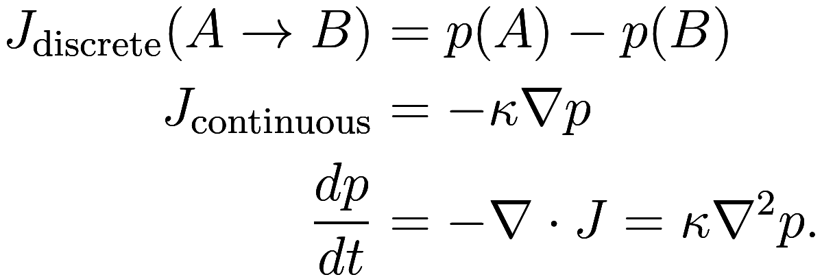If two nodes A and B are connected, then the probability of a random walker at A going to B equals the probability of a random walker at B going to A,³As an example of a more advanced application for random walks, this observation was a key step in my proof of the uniformity of the microcanonical ensemble from my post on negative temperatures so the net rate at which the random walker moves from A to B is controlled only by the difference in probability that it is at A minus the probability it is at B. That is, probability “flows” from A to B in exactly the way heat or any other diffusive process flows:⁴Below, $J$ is the rate of flow of probability (or heat), which is proportional to the gradient in probability $p$ ; then the rate of change of probability at a point is equal to the divergence of $J$ , which is therefore proportional to the Laplacian of $p$ . This is the basic substance of Fourier’s law or the heat equation which governs all diffusive processes.

$\begin{aligned} J_{\text{discrete}}(A \to B) &= p(A) - p(B) \\ J_{\text{continuous}} &= -\kappa \nabla p \\ \frac {dp}{dt} &= -\nabla \cdot J = \kappa \nabla^2 p. \end{aligned}$

Consequentially, the distance traveled from the origin in time $t$ scales like $\sqrt t$ , regardless of dimension. (In a lattice, the position at time $t$ is $P_t = X_1 + \cdots + X_t$ a sum of steps $X_i$ , each of which are iid. In an unbiased random walk the $X_i$ have mean zero, so they are uncorrelated, and therefore the variance $\operatorname{Var}(P_t) = \sum \operatorname{Var}(X_i) = t \operatorname{Var}(X_1)$ grows linearly with $t$ , and the standard deviation is the square root of the variance and grows like $\sqrt t$ . In a biased random walk the bias eventually dominates and distance traveled scales like $t$ .)

Now let us ask: what is the probability that the walker is at the origin at time $t$ ? Let us crudely approximate that at each time $t$ the walker is randomly located in a ball of radius $\sqrt t$ centered at the origin. Such a ball has a volume that scales like $V = t^{d / 2}$ in dimension $d$ , so the chance of being at any particular site is $t^{-d / 2}$ . So the expected number of times for it to strike the origin by time $t$ is

$\int_1^t s^{-d / 2}\ ds \sim \begin{cases} \sqrt t & \text{if } d = 1 \\ \log t & \text{if } d = 2 \\ C - t^{1 - d / 2} & \text{if } d > 2 \end{cases}$

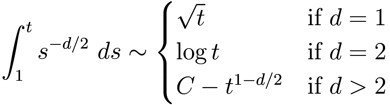
So in one dimension, we are likely to return to the origin again and again (though note: the expected value of the time it takes to return to the origin is infinite!), and above two dimensions the probability of returning to the origin quickly approaches some asymptote; that is, if we return to the origin at all, we probably did so right away, and conversely if we don’t return to the origin quickly, we likely will not return ever.⁵For a more rigorous but readable exposition of the discussion so far see chapter 2.1 of this book on 2D random walks by Serguei Popov, including the key observation that the probability of returning to the origin is 1 if and only if the expected value of the number of returns is infinite. At two dimensions exactly we have a sort of “scale invariance”, and our heuristic is not precise enough to be conclusive.

Now it is possible to analytically determine the probability of returning to the origin (as was first done by Polya in 1921) but let us take an easier approach of computer simulation. Of course, no simulation can directly simulate infinite time, so instead let us numerically estimate the survival function $S(t)$ , which is the probability that at time $t$ the random walk has not yet returned to the origin. Our plan is to infer the behavior of $S(t)$ ⁶in particular, whether or not it is a power law, as power laws are a major focus of this course and then extrapolate the limit $t \to \infty$ .

This is easily done with Monte Carlo simulation. For example, in 1D, we can estimate $S(t)$ by sampling $N$ random walks as follows:

import random
def walk1(N, t):
    count = 0
    for i in range(N):
        pos = 0
        for j in range(t):
            pos += random.choice([-1, 1])
            if pos == 0:
                count += 1
                break
    return (N - count) / N

This is not especially efficient, and we can get a healthy speed boost by using NumPy and vectorizing our computations:

import numpy as np
def walk2(N, d, t):
    r = np.random.choice([-1, 1], size = (N, d, t))
    pos = np.cumsum(r, axis = 2)
    touched_origin = np.any(np.all(pos == 0, axis = 1), axis = 1)
    return (N - np.sum(touched_origin)) / N

Here we have moved up to $d$ dimensions. We first compute all the random numbers we need up front. Integrating along the time axis gives us the position of each of the $N$ random walkers as a function of time. Each such random walker touched the origin if at any time (np.any(..., axis = 1)), all of the coordinates (`np.all(..., axis = 1)) are zero.⁷Yes I had a bug in the first version where I forgot that np.all removed an axis and so used axis = 2 for the time axis.

These simulations are more than sufficient to solve the problem, but we can improve on them. Rather than simulating a finite collection of random walkers, let us track the probability distribution that the random walker is at each point, effectively simulating an infinite number of random walkers. Of course, now we run into the dual difficulty: there are infinitely many possible locations!⁸Note a common programming trick we do not use here (as it is not particularly helpful in this case): one can track the probability distribution in a region near the origin, and a list of individual walkers that go beyond that region, thus combining the two methods with the strengths of each one.

To address this, we will limit ourselves to a square region centered at the origin, and say that any walker that leaves this square region has escaped to infinity, never to return. How large to make this region? Well, in the introduction of the book by Popov linked above, we learn that should we take a 2D random walk starting at the center of the Milky Way⁹ignoring difficulties posed by a certain black hole on a 1 meter lattice, then there is 3.1% chance of that we leave the Milky Way before returning to the starting point. Thus if our square is smaller than $10^{21}$ on a side, we will overestimate the probability of infinite escape by at least 3.1%! This seems pretty bad, but keep in mind that even in 1D the expected value of the time it takes to return to the origin is infinite, but we are only trying to calculate $S(t)$ for “small” times $t$ , so most of those long returns will be at such great times as to be irrelevant. This is the reason we are trying to estimate the shape of $S(t)$ and extrapolate analytically, rather than directly measure $S(\infty)$ by computer.

Okay. How do we update the probability distribution at each time step? With a little thought, we see the probability diffuses exactly following the heat equation / Fourier’s law, say in 3D like:

prob[1:-1, :, :] = 0.5 * (prob[:-2, :, :] + prob[2:, :, :])
prob[:, 1:-1, :] = 0.5 * (prob[:, :-2, :] + prob[:, 2:, :])
prob[:, :, 1:-1] = 0.5 * (prob[:, :, :-2] + prob[:, :, 2:])

Now it becomes an exercise in writing a function that can use NumPy with a variable number of dimensions, so keep the above example in mind:

def walk3(d, t, radius):
    n = 2 * radius + 1
    prob = np.zeros((n,) * d)
    origin = (radius,) * d
    prob[origin] = 1
    touched_origin = np.zeros((t,))

    # Precompute various index slices
    ind_all = slice(None, None)
    ind_low = slice(None, -2)
    ind_high = slice(2, None)
    ind_mid = slice(1, -1)
    ind = [None] * d
    for j in range(d):
        ind[j] = lambda x : (ind_all,) * (j) + (x,) + (ind_all,) * (d - j - 1)

    for i in range(t):
        # Diffuse in each dimension
        for j in range(d):
            prob[ind[j](ind_mid)] = 0.5 * (prob[ind[j](ind_low)] + prob[ind[j](ind_high)])

        if i > 0:
            touched_origin[i] = touched_origin[i - 1] + prob[origin]
        prob[origin] = 0

    return 1 - touched_origin

(At the time I had simply hard-coded the number of dimensions I was simulating, but sometimes variable dimensions with NumPy is useful so I wanted to demonstrate one way to do so.)

Finally, we want to graph the computed survival functions:

def plot_s_d(N, ts, d, radius):
    if d == 1:
        s_w1 = [walk1(N, t) for t in ts]
    s_w2 = [walk2(N, d, t) for t in ts]
    s_w3 = walk3(d, ts[-1], radius)

    y0 = min(np.min(s_w2), np.min(s_w3))
    y1 = np.max(s_w2)

    ts3 = 1 + np.arange(ts[-1])

    plt.clf()
    if d == 1:
        plt.plot(ts, s_w1, label = 'walk1, N = {}'.format(N))
    plt.plot(ts, s_w2, label = 'walk2, N = {}'.format(N))
    plt.plot(ts3, s_w3, label = 'walk3, radius = {}'.format(radius))
    plt.title('Survival function of {}D random walk'.format(d))
    plt.xlim(ts[0] - 1, ts[-1] + 1)
    plt.ylim(y0, y1)
    plt.xlabel('time')
    plt.ylabel('probability of survival')
    plt.yscale('log')
    plt.xscale('log')
    plt.legend(loc = 'upper right')
    plt.savefig('fig_randomwalk_s{}.png'.format(d), dpi = 200)

We make a log-log plot in hopes of revealing a power law, which would appear to be a straight line. What do we find? (Click to enlarge.)

Looks pretty straight to me! Let’s compute a line of best fit¹⁰Note, fitting to power laws is a fraught business that will frequently lead to spurious results if not done with great care, but here our data is so good that we don’t need to think about it. and repeat for each of 1D, 2D, and 3D. Based on our heuristic argument above, these should exhibit all three relevant behaviors, being below, at, and above the critical dimension.

    low = 5

    fit = np.polyfit(np.log(ts3[low:]), np.log(s_w3[low:]), 1)
    a = fit[0]
    b = np.exp(fit[1])
    s_est = b * np.power(ts3[low:], a)
    plt.plot(ts3[low:], s_est, label = 'b * t^a; a = {:.3f}, b = {:.3f}'.format(a, b))
    print('S = b * t^a')
    print('a = ', a, 'b = ', b)
    plt.legend(loc = 'upper right')
    plt.savefig('fig_randomwalk_s{}_fit.png'.format(d), dpi = 200)

Output:

Fit for survival function S(t) = b * t^a in 1 dimensions:
a =  -0.49996732157952334 b =  0.7976891683492726

Fit for survival function S(t) = b * t^a in 2 dimensions:
a =  -0.1056300254846708 b =  0.6728236962323205

Fit for survival function S(t) = b * t^a in 3 dimensions:
a =  -0.005358283923709006 b =  0.7598640873165888

The results:

In 1D we see a very clean power law $S(t) \sim 1 / \sqrt t$ . Taking the limit $t \to \infty$ , we conclude that $S(\infty) = 0$ and the probability that the walker eventually returns to the origin is 100%.

In 2D we again see what looks like it could be a power law, but is that really a straight line? No! There is something of a slight curve to it. From this graph alone we do not have sufficient information to extrapolate behavior at infinite time.

3D looks even less like a power law; from the graph one might guess that $S(t)$ rapidly approaches some asymptote, with a little more than a 70% chance of escape.

We can do better with our 2D results by checking it against results from theory. Equation 2.18 from a 1951 paper by Dvoretzky and Erdos tells us that

$S_2(t) = \frac \pi{\log t} + O\left(\frac {\log \log n}{\log^2 n}\right)$

and indeed we observe a very good fit for $1 / S_2(t)$ as a linear function of $\log t$ :

though the constants are not accurate enough for us to confirm the theoretical value of $a = \pi$ :¹¹The values of the constants depend not just on the dimension of the graph, but on its shape and the distribution of the walker’s steps, so one has to check that we are using the same definition of a random walk as Dvoretzky and Erdos. Interestingly the standard 2D random walk is in fact the same as two simultaneous, independent 1D random walks, if you rotate the coordinate axes by 45 degrees.

Fit for survival function S(t) = a / (log(t) + b) in 2 dimensions:
a =  3.2450755245666127 b =  3.2064465739692407

As expected, $S_2(t) \to 0$ (extremely slowly) in the limit $t \to \infty$ , so the probability of eventually returning to the origin is 100%. While we were able to numerically validate the theoretical result, note that doing so is quite finicky – trying to fit $S(t)$ as a linear function of $1 / \log t$ gives a result about equally as bad as the power law had.

Novel to me, anyhow – I am presumably not the first to compute the fractal dimensions of spirals, say, even if I could not find any precedent.↩︎
a deficiency shared by many of my students↩︎
As an example of a more advanced application for random walks, this observation was a key step in my proof of the uniformity of the microcanonical ensemble from my post on negative temperatures ↩︎
Below, $J$ is the rate of flow of probability (or heat), which is proportional to the gradient in probability $p$ ; then the rate of change of probability at a point is equal to the divergence of $J$ , which is therefore proportional to the Laplacian of $p$ . This is the basic substance of Fourier’s law or the heat equation which governs all diffusive processes.↩︎
For a more rigorous but readable exposition of the discussion so far see chapter 2.1 of this book on 2D random walks by Serguei Popov, including the key observation that the probability of returning to the origin is 1 if and only if the expected value of the number of returns is infinite.↩︎
in particular, whether or not it is a power law, as power laws are a major focus of this course↩︎
Yes I had a bug in the first version where I forgot that np.all removed an axis and so used axis = 2 for the time axis.↩︎
Note a common programming trick we do not use here (as it is not particularly helpful in this case): one can track the probability distribution in a region near the origin, and a list of individual walkers that go beyond that region, thus combining the two methods with the strengths of each one.↩︎
ignoring difficulties posed by a certain black hole↩︎
Note, fitting to power laws is a fraught business that will frequently lead to spurious results if not done with great care, but here our data is so good that we don’t need to think about it.↩︎
The values of the constants depend not just on the dimension of the graph, but on its shape and the distribution of the walker’s steps, so one has to check that we are using the same definition of a random walk as Dvoretzky and Erdos. Interestingly the standard 2D random walk is in fact the same as two simultaneous, independent 1D random walks, if you rotate the coordinate axes by 45 degrees.↩︎

Follow RSS/Atom feed for updates.