(As mentioned before, current MIT students should not read this material.)
If you tried to compare the lengths of the coastlines of different countries, you would find that different sources give wildly contradictory results. For example, The World Factbook says the coastline of Norway is more than 4 times as long as that of the US, while the World Resources Institute says the US coastline is almost 3 times as long. These two sources disagree on the total length of coastline in the world by a factor of 5!
The coastline paradox says that the length of a coastline depends on the scale at which the measurement is taken. A one-dimensional object has a length that scales linearly with its size, and a two-dimensional object has an area that scales quadratically with size; coastlines, however, typically have a measure that varies with size in a power law with power between 1 and 2. Such an object has “fractional dimension”, ie is a fractal.
There are several ways to define the dimension of a fractal (and in rare cases they disagree!); we will use the box counting definition. This is the same definition we used to measure the dimension of fractal spirals.
For some ![]() , let us cover the coastline (or other object) with
boxes with side length
, let us cover the coastline (or other object) with
boxes with side length ![]() .1The
boxes could be 2D, 3D, etc., according to the dimension of the space the
fractal is embedded in. Let
.1The
boxes could be 2D, 3D, etc., according to the dimension of the space the
fractal is embedded in. Let ![]() be the number of boxes of size
be the number of boxes of size ![]() required. Then the dimension
required. Then the dimension ![]() is defined by
is defined by
![]()
We will shortly be computing ![]() for various
for various ![]() , but if we tried to directly apply this formula we
would get a very poor answer. Instead let us anticipate that we may find
, but if we tried to directly apply this formula we
would get a very poor answer. Instead let us anticipate that we may find
![]() follows a power-law, such as
follows a power-law, such as ![]() . Then
. Then
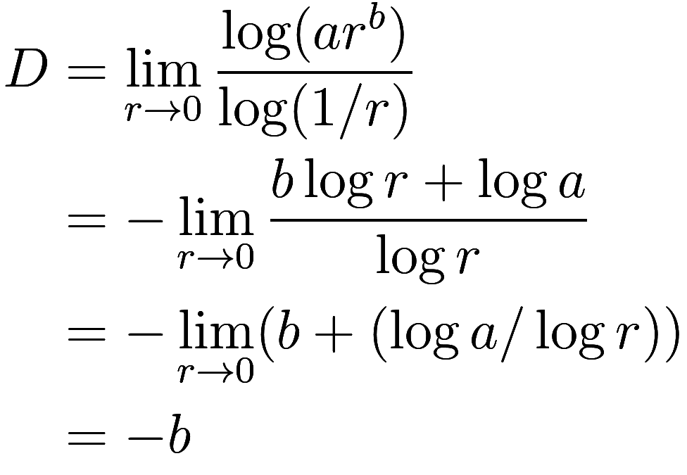
as when ![]() ,
, ![]() .
.
Let us apply this to the coastline of Massachusetts. Raw GIS data is available here; from this we can extract a list of 200 thousand (x, y) coordinates, in meters (I think).2Students were provided with this text file. Generally data points are spaced at an interval of about 50 meters apart:
We compute ![]() for 1000 values of
for 1000 values of ![]() , spaced linearly in log space:
, spaced linearly in log space:
import numpy as np
xys = []
with open('mass_coastline', 'r') as f:
    for line in f:
        x, y = line.split()
        xys.append((float(x), float(y)))

rs = np.exp(np.linspace(np.log(1), np.log(1e7), 1000))
ns = np.zeros(rs.shape)
for i in range(np.size(rs)):
    r = rs[i]

    s = set()
    for x, y in xys:
        s.add((int(x / r), int(y / r)))
    ns[i] = len(s)

i = (rs > 1e2) & (rs < 1e5)
a_, b_ = np.polyfit(np.log(rs[i]), np.log(ns[i]), 1)
Fitting a power-law, we find:
![]() is an excellent fit to a power-law across
three orders of magnitude! We find that the Massachusetts coastline
consistently has a fractal dimension of
is an excellent fit to a power-law across
three orders of magnitude! We find that the Massachusetts coastline
consistently has a fractal dimension of ![]() .
.
What would have happened if, instead of fitting ![]() to a power law and taking the exponent, we had
naively applied the definition of
to a power law and taking the exponent, we had
naively applied the definition of ![]() directly? When taking the limit, we would have to
stop around
directly? When taking the limit, we would have to
stop around ![]() meters, as below that the fit degrades
quickly. At that scale we have
meters, as below that the fit degrades
quickly. At that scale we have ![]() , so
, so
![]()
which is quite wrong. In fact we don’t even get a positive
dimension until ![]() is below 1 meter. This should be suspicious: why
does our result depend on the units that we measure
is below 1 meter. This should be suspicious: why
does our result depend on the units that we measure ![]() in? If we instead had
in? If we instead had ![]() km, we’d at least get a positive number for
the dimension (namely 4.588, still very wrong). Indeed, in our
definition for
km, we’d at least get a positive number for
the dimension (namely 4.588, still very wrong). Indeed, in our
definition for ![]() , the value inside the limit does depend on the
choice of units of
, the value inside the limit does depend on the
choice of units of ![]() ! But the value of the limit, if that
limit exists, does not depend on the units of
! But the value of the limit, if that
limit exists, does not depend on the units of ![]() , so the definition is well-defined.
, so the definition is well-defined.
Finally, observe that there are actually three different power-laws
we could fit to ![]() , depending on the range of
, depending on the range of ![]() we use. For
we use. For ![]() smaller than about 10 meters, we find that the
coastline is zero-dimensional; this is because around that scale the raw
coastline data can be resolved into a collection of individual points.
(If we had connected points with lines we would instead find the
coastline to be one-dimensional at this scale.) And then for
smaller than about 10 meters, we find that the
coastline is zero-dimensional; this is because around that scale the raw
coastline data can be resolved into a collection of individual points.
(If we had connected points with lines we would instead find the
coastline to be one-dimensional at this scale.) And then for ![]() above
above ![]() meters we again see the coastline is
zero-dimensional; this is because the entire coastline fits into a
single box, and at this scale appears to be a single point.
meters we again see the coastline is
zero-dimensional; this is because the entire coastline fits into a
single box, and at this scale appears to be a single point.
Follow RSS/Atom feed for updates.